5 Ways to Display Cells from Another Sheet in Excel

The ability to display cells from another sheet in Excel is an incredibly powerful tool that can significantly enhance your data management and analysis capabilities. Whether you're managing large datasets, creating comprehensive reports, or simply organizing your information, knowing how to reference and display data from multiple sheets within one workbook can streamline your workflow, reduce redundancy, and keep your data synchronized. Here are five methods to seamlessly connect your data across sheets in Excel:
1. Cell References

The simplest and most common way to reference data from another sheet is through direct cell references. Here's how you do it:
- Click the cell where you want the data to appear.
- Start typing the equal (=) sign.
- Click on the tab of the sheet where the data resides.
- Select the cell you want to reference. Excel will automatically generate the reference in the formula bar, e.g., =Sheet2!A1
⚠️ Note: Make sure the sheet name does not contain spaces, or wrap it in single quotes in the formula, e.g., ='Sheet Two'!A1.
2. Named Ranges

Using named ranges makes formulas easier to understand, especially when dealing with complex spreadsheets. Here are the steps:
- Go to the source sheet, select the range you want to name.
- Right-click and choose "Define Name..." or press Ctrl + F3, then click "New".
- Name your range and press OK.
- In your destination sheet, you can now reference this range with the name you provided, e.g., =Sheet2!NamedRange
3. Using INDEX and MATCH

If you need to look up values from another sheet based on certain criteria, using the combination of INDEX and MATCH functions can be highly effective:
- INDEX will return the value of a cell in a table based on the row and column numbers.
- MATCH will look for a value in an array and return its position.
=INDEX(Sheet2!$A$1:$E$100,MATCH($A2,Sheet2!$A$1:$A$100,0),2)
4. VLOOKUP or HLOOKUP

Another popular lookup method involves using VLOOKUP or HLOOKUP functions:
- VLOOKUP searches for a value in the first column of a table and returns a value in the same row from another column.
- HLOOKUP works similarly but searches for the value across the top row instead.
=VLOOKUP($B$1,Sheet2!$A$1:$E$100,2,FALSE)
5. Power Query

For more advanced Excel users, Power Query provides a robust solution for combining data from multiple sheets:
- Go to the Data tab and select "Get Data" > "From File" > "From Workbook".
- Navigate to and select your Excel workbook, then choose the sheets you want to connect.
- Use the interface to combine data as needed, either by appending or merging queries.
- Load the combined data into your current worksheet.
💡 Note: Power Query is available in Excel 2010 and later versions.
Summary

Mastering these techniques will allow you to efficiently manage and analyze data across multiple sheets, enhancing your productivity and reducing the risk of errors. Each method has its place depending on the complexity of your data needs, from simple cell references to sophisticated data transformations with Power Query. Remember, the key to effective data management in Excel is understanding when and how to leverage these features for your specific tasks.
Can I reference multiple cells at once from another sheet?

+
Yes, you can reference multiple cells by selecting a range. For example, =Sheet2!A1:A10 would reference cells A1 through A10 from Sheet2.
How do I make my references dynamic?

+
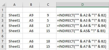
Use named ranges or functions like OFFSET and INDIRECT to create dynamic references that adjust automatically when new data is added or when the structure of your workbook changes.
What happens if I delete the sheet referenced in my formulas?

+
If you delete or rename the source sheet, Excel will show #REF! errors where the formulas were trying to pull data from the now missing or renamed sheet.


