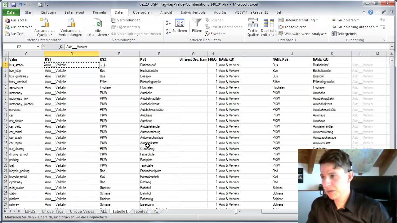
Creating a Dropdown Menu in Excel: Easy Steps

Excel is a powerhouse tool when it comes to data organization and manipulation, offering various functionalities that can streamline your work. One such feature is the ability to create dropdown menus, which greatly enhances data entry accuracy and efficiency by providing predefined selections. Let's dive into how you can create your own dropdown menu in Excel, following simple steps.
Understanding Dropdown Menus

Before we get into the steps, let's briefly understand what a dropdown menu is. A dropdown menu, or list, in Excel allows users to choose from a set of pre-filled options in a cell. This not only reduces errors in data entry but also ensures uniformity in input. Here's how you can add this functionality to your spreadsheets:
Steps to Create a Dropdown Menu in Excel

1. Preparing Your List Data

- Identify or create the list of items you want to include in your dropdown menu.
- Place this list in a separate area of your worksheet or on a different sheet entirely.
2. Using Data Validation

- Select the cell where you want the dropdown list to appear.
- Go to the Data tab, and under the Tools group, click on Data Validation.
- In the Data Validation dialog box, under the Settings tab, change Allow to List.
- In the Source field, either type the list directly, or select your list range from the sheet by clicking the small arrow to collapse the box and then dragging over your data.
- Click OK to apply the settings.
3. Adjusting Dropdown Settings

- Once your dropdown list is created, you can further customize the behavior:
- Go back into the Data Validation settings to allow blank or prevent invalid entries.
- You can also add input messages to guide users and error alerts for incorrect entries.
⚠️ Note: If your list is on a different sheet, reference it like this: =Sheet2!A1:A10
Expanding Dropdown Functionality

1. Dynamic Ranges

- To make your dropdown list update automatically when you add or remove items from your source list, use named ranges with OFFSET and COUNTA functions.
- Create a named range for your list, then update the Data Validation Source to reference this named range.
2. Dropdown Based on Another Cell

- You can set up dependent dropdowns where the options in one dropdown depend on the selection made in another. This involves setting up lists in separate ranges and using the INDIRECT function in the Data Validation source.
💡 Note: For dependent dropdowns, ensure the first list's options match the names of the dependent lists' ranges.
Table of Example Data

| Dropdown Type | Example Source Range | Data Validation Source |
|---|---|---|
| Static List | A1:A5 | =Sheet1!A1:A5 |
| Dynamic List | =OFFSET(Sheet1!A1,0,0,COUNTA(Sheet1!A:A),1) | =DynamicRangeName |
| Dependent List | A1:A5 (Categories), B1:B5 (Subcategories) | =INDIRECT(A1) |

Incorporating dropdown menus into your Excel sheets can significantly enhance data entry, organization, and analysis. They offer consistency, reduce errors, and make your spreadsheets more user-friendly. Whether you're tracking inventory, creating surveys, or managing project tasks, dropdowns can be a valuable tool in your Excel toolkit.
Can I change the dropdown list based on another cell’s value?

+
Yes, you can use dependent dropdown lists by setting up ranges named after items in a first dropdown, then use the INDIRECT function in Data Validation.
How do I make the dropdown list update automatically?

+
Create a named range using OFFSET and COUNTA functions to dynamically update the list as items are added or removed.
What if I want to allow users to type their own entries?

+
In the Data Validation settings, you can uncheck the “Ignore blank” option or set the List option to include a blank option to allow manual entry.


