5 Ways to Link Cells Between Sheets in Excel
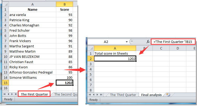
Linking cells between sheets in Excel can streamline your work, allowing you to manage data across different tabs efficiently. Whether you're compiling a report, creating a dashboard, or simply organizing vast amounts of data, knowing how to link cells can save time and reduce errors. Here are five methods to achieve this, ensuring your spreadsheets are more interconnected and functional.
1. Direct Cell References

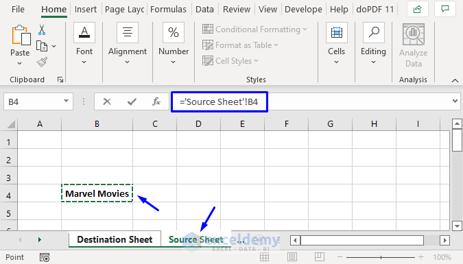
The simplest way to link cells between sheets is through direct cell references. This method lets you reference a cell from another sheet in your current sheet.
- Step 1: Click on the cell where you want the linked data to appear.
- Step 2: Enter the equal sign (=) to start the formula.
- Step 3: Click on the sheet tab where your source data is located. The cell reference will automatically include the sheet name, like
Sheet2!A1if you’re pulling data from cell A1 in Sheet2. - Step 4: Finish by pressing Enter. The cell will now display the value or formula result from the source cell.
Example: =Sheet2!A1 will pull the content from cell A1 in Sheet2 into your current cell.
💡 Note: Changes in the source cell automatically update the linked cell, ensuring your data remains current.
2. 3D References
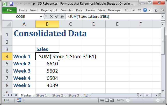
If you have similar data across multiple sheets, 3D references can be useful. This method aggregates data from the same cell across different sheets.
- Step 1: Select the cell where you want to summarize the data.
- Step 2: Enter the formula using the SUM function (or any other function that makes sense for your data), like
=SUM(Sheet1:Sheet3!A1)if you’re summing up cell A1 from Sheets 1 to 3.
This formula will sum the values from cell A1 across all sheets named Sheet1 to Sheet3.
📊 Note: 3D references are especially handy for creating summaries or roll-ups of similar data points across sheets.
3. Using Named Ranges
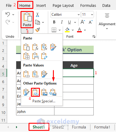
Creating named ranges can make your formulas easier to understand and maintain when linking data across sheets.
- Step 1: Go to the source sheet, select the range of cells you want to link.
- Step 2: Navigate to Formulas > Define Name, or press Ctrl+F3, to name the range (e.g.,
SalesData). - Step 3: In your destination sheet, use the named range in your formula, like
=SUM(SalesData). This will automatically link to the named range on the source sheet.
Example: If you named a range SalesData on Sheet2, you can reference it in any other sheet as =SalesData.
🏷️ Note: Named ranges make your spreadsheets more readable and easier to manage, especially in complex workbooks.
4. Hyperlinks

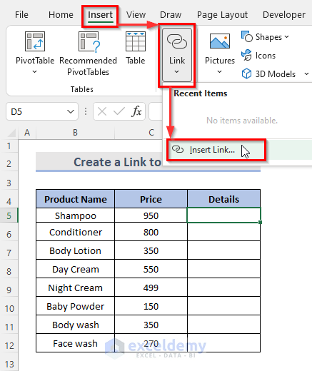
Hyperlinks are another way to link cells, especially useful for navigation within your workbook.
- Step 1: Right-click the cell where you want to place the hyperlink.
- Step 2: Select ‘Hyperlink’ and choose ‘Place in This Document.’
- Step 3: Select the cell or range on another sheet, and set the display text as needed.
Example: If you want a cell to link to cell A1 on Sheet3, you would type in Sheet3!A1 and set the display text to something like “Go to Sheet3 Data”.
🔗 Note: Hyperlinks can be visually represented with underlining or different coloring, making it intuitive to navigate your Excel workbook.
5. VLOOKUP or HLOOKUP Across Sheets

For more complex linking scenarios where you need to retrieve data based on certain conditions or keys, VLOOKUP or HLOOKUP can be employed across sheets.
- Step 1: In the cell where you want the lookup result, start by typing
=VLOOKUP(. - Step 2: Provide the lookup value, the table array from another sheet, the column index number, and the range lookup (TRUE for approximate match, FALSE for an exact match).
Example: =VLOOKUP(A1, Sheet2!A1:B100, 2, FALSE) will look for the value in A1 of the current sheet in the first column of the table array in Sheet2, returning the corresponding value from the second column.
🔎 Note: VLOOKUP is particularly useful for databases or tables split across sheets where you need to look up data based on unique identifiers.
In conclusion, linking cells between sheets in Excel provides numerous benefits, enhancing your data management capabilities. By mastering these five methods, you can create dynamic, interconnected spreadsheets that automatically update, reduce redundancy, and maintain data integrity across your workbook. Each method has its use case, from simple direct references to more advanced techniques like 3D references or complex lookups. Remember to keep your spreadsheet clean and organized to maximize the effectiveness of these linking techniques, making your data not just organized but also insightful and actionable.
Can I link cells across different workbooks?
+
Yes, you can link cells between different Excel workbooks using an external reference. The formula would look something like =[Book2.xlsx]Sheet1!A1, where Book2.xlsx is the name of the external workbook.
What happens if I rename or delete the source sheet?

+
If you rename the source sheet, Excel will update the references automatically. However, if you delete the source sheet, linked formulas will return #REF! errors, indicating a broken link.
How can I manage large spreadsheets with multiple links effectively?
+
Using named ranges, organizing your data logically, and employing VLOOKUP or other advanced functions can help manage large spreadsheets with multiple links. Also, consider using Power Query for external data management.
