How To Find Duplicates In Excel Between Two Sheets

Working with Excel can be a powerful way to organize and analyze data, especially when dealing with large datasets spread across multiple sheets. One common task that many users face is identifying duplicate values between two different sheets within the same workbook. This task can be crucial for data cleaning, merging, or validating data entries to avoid redundancy and ensure data integrity. Here, we'll walk through a step-by-step guide on how to find and manage duplicates effectively in Excel.
Understanding Duplicates in Excel
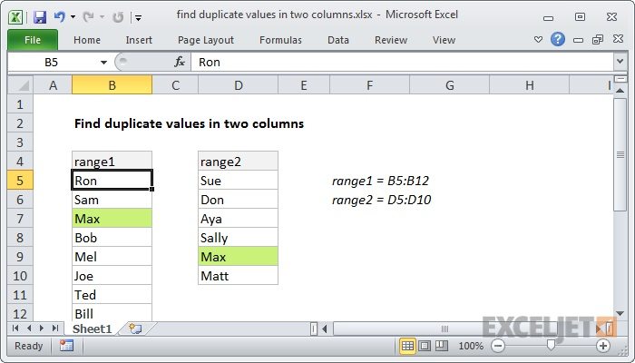
Duplicates in Excel can refer to:
- Identical values in the same column or row
- Repeated sets of data across different rows
These duplicates might occur due to data entry errors, data merging from different sources, or simply oversight. The key is to recognize and handle these effectively.
Preparation Before Finding Duplicates
Before diving into the process:
- Ensure both sheets have a common column to compare. This could be an ID, a name, or any unique identifier.
- Check for data consistency (format, spelling, etc.) across sheets to avoid overlooking duplicates due to minor variations.
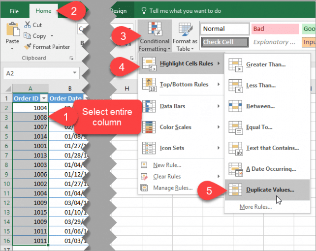
Method 1: Conditional Formatting to Highlight Duplicates

Excel’s conditional formatting offers a visual approach to spot duplicates:
- Navigate to the first sheet: Go to Home > Conditional Formatting > New Rule.
- Select the rule type: Choose ‘Use a formula to determine which cells to format.’
- Enter the formula:
=COUNTIF(Sheet2!A1:A1000, A1) > 0
This assumes ‘A1’ is your unique identifier column, and Sheet2 contains the data you’re comparing against. Adjust the range as needed. - Set the formatting: Choose a fill color or font style to highlight the duplicates.
- Apply: Click ‘OK’ and apply this rule to all cells in the column you’re checking for duplicates.
🔍 Note: This method is best for visual identification rather than for further data processing.
Method 2: Using VLOOKUP for Identifying Duplicates

VLOOKUP is another tool that can be used for finding duplicates:
- Prepare the destination: In Sheet1, create a new column next to your data (say column B) for results.
- Set up VLOOKUP:
=IF(ISERROR(VLOOKUP(A1, Sheet2!A1:A1000, 1, FALSE)), “Unique”, “Duplicate”)
Where A1 is the cell to check for duplicates, and the formula checks against Sheet2’s first column. - Copy down: Drag the formula down to apply it to all entries in your sheet.
This method will label each entry as “Unique” or “Duplicate”.
| Column A (Sheet1) | Column B (Result) |
|---|---|
| Entry1 | Unique |
| Entry2 | Duplicate |
| … | … |

🔎 Note: VLOOKUP is an excellent way to not only identify but also to manage duplicates programmatically within Excel.
Method 3: Advanced Filter for Duplicate Entries
For more complex scenarios, use Excel’s Advanced Filter:
- Select the data: Highlight the entire column or range containing your data in Sheet1.
- Go to Data tab: Choose ‘Advanced’ under the Filter section.
- Configure filter:
- Select ‘Copy to another location’
- Choose the list range (where your data is located)
- Enter a location where you want duplicates copied to
- Check ‘Unique records only’
- Apply filter: Click ‘OK’. This will show unique entries, and you can then isolate duplicates manually.
💡 Note: This method is useful when you want to physically separate duplicates from your main dataset.
Automating with VBA for Massive Data Sets

If you frequently deal with very large datasets, VBA scripts can automate the process:
- Open VBA editor: Press Alt + F11 to open the Visual Basic Editor.
- Insert a new module: Right-click any object in Project Explorer > Insert > Module.
- Write the script:
Sub FindDuplicates() Dim ws1 As Worksheet, ws2 As Worksheet Set ws1 = Sheets(“Sheet1”) Set ws2 = Sheets(“Sheet2”)This script will highlight duplicates in Sheet1 based on the entries in Sheet2.Dim lastRow1 As Long, lastRow2 As Long lastRow1 = ws1.Cells(ws1.Rows.Count, "A").End(xlUp).Row lastRow2 = ws2.Cells(ws2.Rows.Count, "A").End(xlUp).Row Dim rng1 As Range, rng2 As Range Set rng1 = ws1.Range("A1:A" & lastRow1) Set rng2 = ws2.Range("A1:A" & lastRow2) For Each cell In rng1 If WorksheetFunction.CountIf(rng2, cell.Value) > 0 Then cell.Interior.Color = RGB(255, 200, 200) ' Red background for duplicates End If Next cellEnd Sub
⚙️ Note: VBA scripts provide a powerful way to automate repetitive tasks in Excel, especially for large datasets.
In conclusion, identifying duplicates between two sheets in Excel can be approached through several methods, each with its own advantages. Whether you choose the visual appeal of Conditional Formatting, the programmatic control of VLOOKUP, the isolation capability of Advanced Filter, or the automation of VBA, Excel offers versatile tools to manage your data effectively. By understanding these techniques, you can ensure your datasets are clean, accurate, and ready for further analysis or integration into other systems. Always consider the scale of your data and the nature of your analysis when choosing the best method for your needs.
Can you identify duplicates across multiple columns?
+
Yes, while the methods described focus on single-column comparisons, you can extend them to work across multiple columns by adjusting the formulas or VBA scripts to compare ranges or by using array formulas.
What if my data has different formats or case sensitivity?

+
Excel’s functions like VLOOKUP and Conditional Formatting can be sensitive to case and format differences. You might need to preprocess your data by using functions like LOWER(), UPPER(), or TRIM() to standardize entries before comparison.
How can I remove duplicates once identified?

+
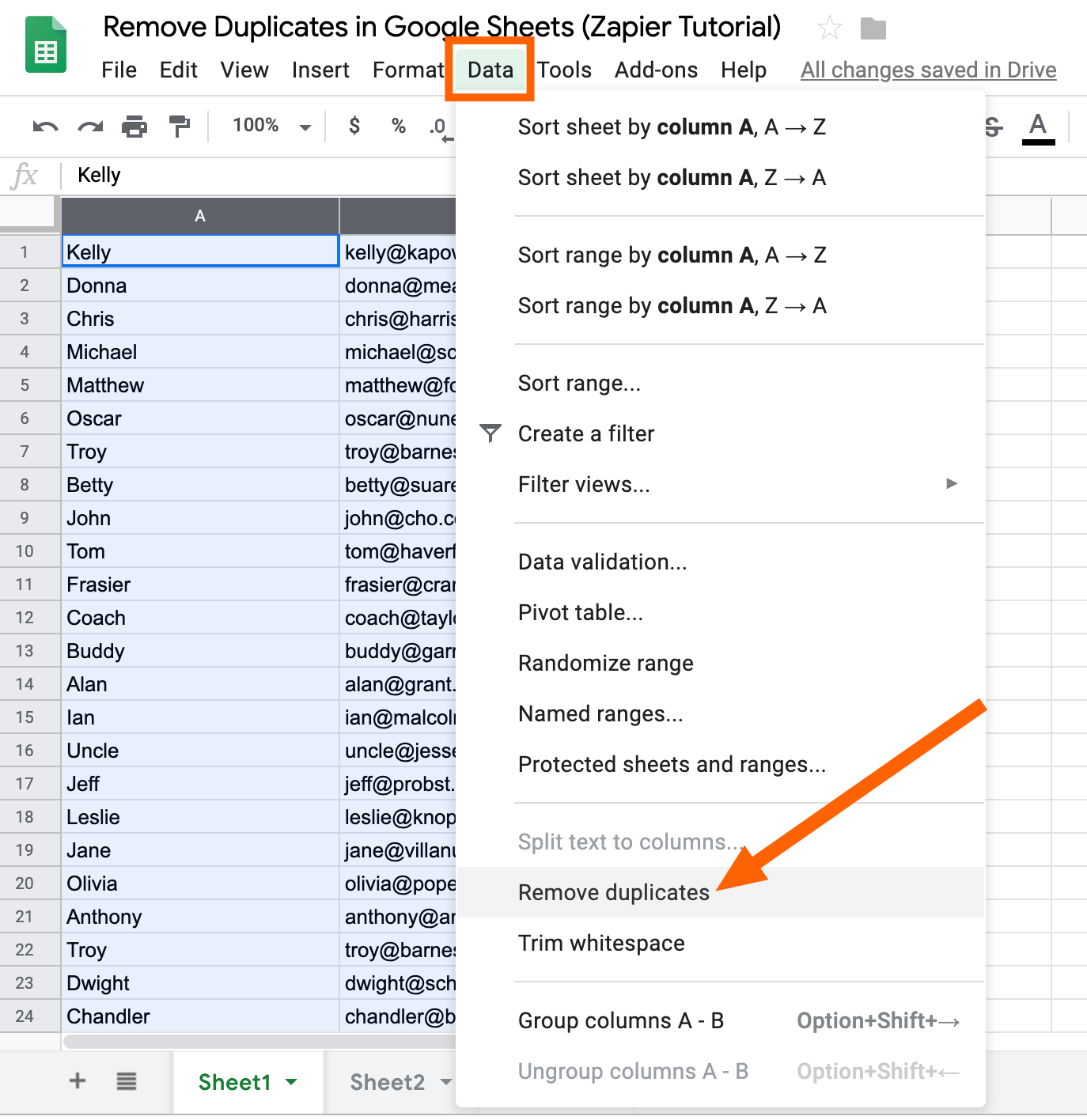
Once duplicates are identified, you can use Excel’s built-in “Remove Duplicates” feature under the Data tab, or manually delete rows if you’ve isolated them with the Advanced Filter or other methods.
