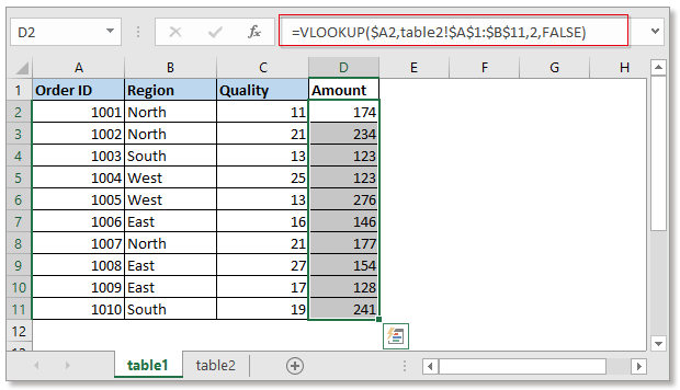
5 Simple VLOOKUP Tips for Two Excel Sheets

If you're managing complex data sets in Excel, mastering the VLOOKUP function can significantly streamline your work, especially when dealing with multiple sheets. Here, we'll delve into five simple yet powerful VLOOKUP tips that will help you efficiently cross-reference data between two Excel sheets. Whether you're a beginner or someone looking to refine your Excel skills, these tips will enhance your data management capabilities.
VLOOKUP Basics

Before diving into advanced tips, let’s ensure you have a solid understanding of what VLOOKUP does:
- Looks for a value in the first column of a specified range,
- Then returns a value from the same row of another column within that range.
- Syntax:
=VLOOKUP(lookup_value, table_array, col_index_num, [range_lookup])

Tip 1: Use Exact Match

To ensure you get the exact match you need:
- Use
FALSEfor the[range_lookup]parameter in VLOOKUP. - This tells Excel to look for an exact match rather than an approximate one.
🔍 Note: Using FALSE helps prevent issues with similar values that are not an exact match.
Tip 2: Reference a Cell for Lookup Value

To make your VLOOKUP formula dynamic:
- Instead of directly typing the lookup value, reference a cell:
=VLOOKUP(C2, Sheet2!A:B, 2, FALSE)
This allows you to change the lookup value simply by altering the content of the referenced cell.
Tip 3: Dealing with Errors with IFERROR

To handle errors gracefully:
- Use the IFERROR function alongside VLOOKUP:
=IFERROR(VLOOKUP(C2, Sheet2!A:B, 2, FALSE), “Not Found”)
This formula will return “Not Found” instead of an error if the lookup value is not in the first column of the specified range.
Tip 4: Using Named Ranges

Named ranges can make your formulas more readable and manageable:
- Name your range:
Sheet2!A:B could be named DataSheet=VLOOKUP(C2, DataSheet, 2, FALSE)
📝 Note: Named ranges not only improve readability but also reduce errors when referencing data.
Tip 5: Speed Up with Approximate Match

For large datasets where an approximate match is acceptable:
- Set the
[range_lookup]parameter to TRUE. - This method is faster but only works if your table is sorted in ascending order by the lookup column.
=VLOOKUP(C2, DataSheet, 2, TRUE)
🚀 Note: Use approximate match when performance matters over precision, but ensure your data is sorted appropriately.
By implementing these VLOOKUP tips, you can increase the efficiency, accuracy, and flexibility of your data analysis across two Excel sheets. Remember, the key to mastering Excel functions like VLOOKUP lies in understanding the context of your data and choosing the right approach for your specific needs.
What is the difference between using TRUE and FALSE in VLOOKUP?

+
When you set range_lookup to TRUE, VLOOKUP will look for an approximate match, assuming the first column of your lookup table is sorted in ascending order. With FALSE, VLOOKUP seeks an exact match.
How can I avoid errors in VLOOKUP when the lookup value is not in the list?

+
You can use the IFERROR function to replace the error with a friendly message or a custom result. For example, =IFERROR(VLOOKUP(C2, DataSheet, 2, FALSE), “Value Not Found”).
Is it possible to use VLOOKUP for multiple sheets?

+
Yes, you can use VLOOKUP to reference data across multiple sheets by specifying the sheet name in the formula. For instance, =VLOOKUP(A2,Sheet1!A:B,2,FALSE) or with named ranges =VLOOKUP(A2,DataSheet,2,FALSE).


