5 Ways to Vlookup from Another Sheet in Excel

When working with large datasets in Excel, it's common to split information across multiple sheets to keep your work organized and efficient. One of the Excel functions that becomes indispensable in such scenarios is VLOOKUP. This function allows you to search for a value in one column of a table and return a corresponding value from another column. Here are five ways you can use VLOOKUP to pull data from another sheet in Excel:

1. Basic VLOOKUP from Another Sheet

The simplest form of VLOOKUP is to reference data from another sheet. Here's how you can do it:

• Open your Excel workbook.
• Click on the cell where you want the VLOOKUP result to appear.
• Type the formula: =VLOOKUP(lookup_value, range, column_index_num, [range_lookup])
• Instead of selecting a range from the current sheet, click on another sheet and select the range. For example:

  =VLOOKUP(A2, Sheet2!A1:B100, 2, FALSE)
  

  Here, A2 is the lookup value from your current sheet, Sheet2!A1:B100 is the lookup range from another sheet, 2 specifies the column from which to return the value, and FALSE ensures an exact match.

🔍 Note: Ensure the lookup table in the other sheet is in ascending order for VLOOKUP to work correctly when not using exact match.

2. Using Named Ranges for Clarity

Instead of hardcoding sheet names and ranges, use named ranges for easier readability and management:

• Go to the source sheet, highlight the range, right-click, and choose "Define Name".
• Name your range (e.g., "Products").
• In your VLOOKUP formula, use the named range:

  =VLOOKUP(A2,Products,2,FALSE)
  

This method simplifies formula creation and maintenance, especially when dealing with large datasets or frequent sheet name changes.

3. VLOOKUP with Dynamic Sheet References

If you need to lookup values from different sheets dynamically, you can use the INDIRECT function:

• Create a dropdown list or cell where you type the sheet name.
• Use this cell reference in the VLOOKUP formula combined with the INDIRECT function to change the lookup table dynamically:

  =VLOOKUP(A2,INDIRECT("'"&B1&"'!"&A1:B100),2,FALSE)
  

  Here, B1 contains the name of the sheet you want to pull data from, and A1:B100 is the range on that sheet.

🔗 Note: The INDIRECT function turns a text string into a cell reference. Be careful with sheet names containing spaces or special characters; enclose them in single quotes.

4. Combining VLOOKUP with MATCH for Column Reference

When dealing with datasets where column numbers might change, you can use the MATCH function within VLOOKUP to dynamically find the correct column:

• Suppose column headers are not static. Use MATCH to find the column number:

  =VLOOKUP(A2,Sheet2!A1:B100,MATCH("Price",Sheet2!A1:B1,0),FALSE)
  

  Here, MATCH("Price",Sheet2!A1:B1,0) finds the column number of "Price".

This method is especially useful when your data structure changes or when you work with datasets where column positions might differ between sheets.

5. VLOOKUP with a Helper Column for Complex Matches

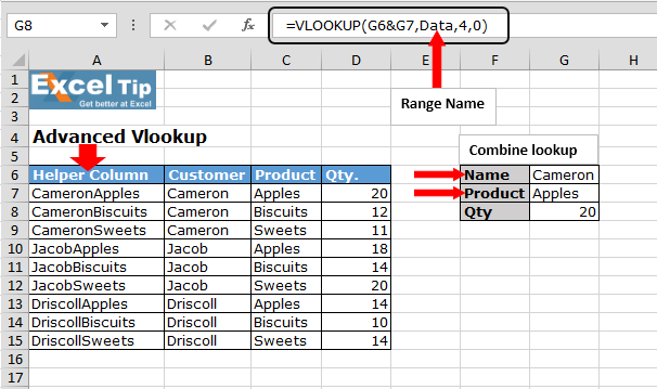
If your lookup involves multiple criteria, create a helper column:

• In the source sheet, create a new column combining unique identifiers (e.g., product ID and year).

  =A2&B2
  

• In your target sheet, concatenate the same criteria in a cell to use as the lookup value:

  =A2&B2
  

  Then use this in your VLOOKUP:

  =VLOOKUP(A2&B2,Sheet2!A1:C100,3,FALSE)
  

This technique simplifies complex lookups and reduces the chance of errors due to misaligned data.

These methods provide you with a variety of ways to use VLOOKUP in Excel, adapting to different scenarios and data structures. VLOOKUP is powerful, but when used across multiple sheets, understanding how to reference and manipulate data effectively can significantly enhance your productivity.

Frequently Asked Questions

Can I use VLOOKUP to return data from multiple sheets at once?

+

VLOOKUP can only return data from one table at a time. However, you can nest multiple VLOOKUPs or use INDEX and MATCH functions for a multi-sheet lookup.

How can I update the source sheet without affecting my VLOOKUP results?

+

If you’re using absolute cell references (e.g., A1:B100), your VLOOKUP formula won’t change. However, ensure the structure of your source sheet remains consistent or update the formula accordingly.

What is the alternative to VLOOKUP for searching left in a table?

+

Use the INDEX and MATCH combination to lookup values to the left. For example:

        =INDEX(Sheet2!A1:A100,MATCH(B2,Sheet2!B1:B100,0))