5 Easy Steps to Unhide Rows in Excel Sheet

Hiding rows in an Excel sheet can help you declutter your workspace, focusing only on the data relevant to your task at hand. However, there comes a time when those rows need to be brought back into view. Whether you are auditing financial reports, tracking project progress, or managing data for a presentation, knowing how to unhide rows in Excel is essential for effective spreadsheet management. This article will guide you through five straightforward methods to unhide rows in Excel, ensuring your workflow remains smooth and uninterrupted.
Using the Context Menu

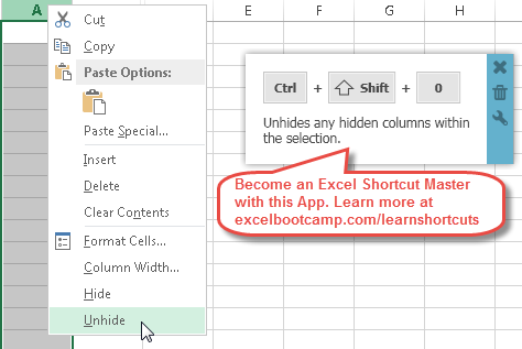
The simplest method to unhide rows involves right-clicking:
- Select the rows surrounding the hidden ones by clicking on their row numbers.
- Right-click to bring up the context menu.
- Click Unhide to reveal the hidden rows.
💡 Note: This method is user-friendly and doesn’t require any special knowledge of Excel.
Keyboard Shortcut Method

If you’re looking for a quick way without using the mouse, the keyboard is your ally:
- Click on the row number above the hidden row(s).
- Hold down the Ctrl key and click the row number below the hidden row(s).
- Press Ctrl + Shift + 9 to unhide.
🎹 Note: Using shortcuts can speed up your work, making it an efficient choice for power users.
The Name Box Technique

For those who prefer using Excel’s built-in features, the Name Box provides an easy way to pinpoint and unhide rows:
- Click into the Name Box located to the left of the formula bar.
- Type in the range that includes the hidden rows, like A3:A5 if you know rows 4 and 5 are hidden.
- Press Enter to select the range, then right-click and choose Unhide.
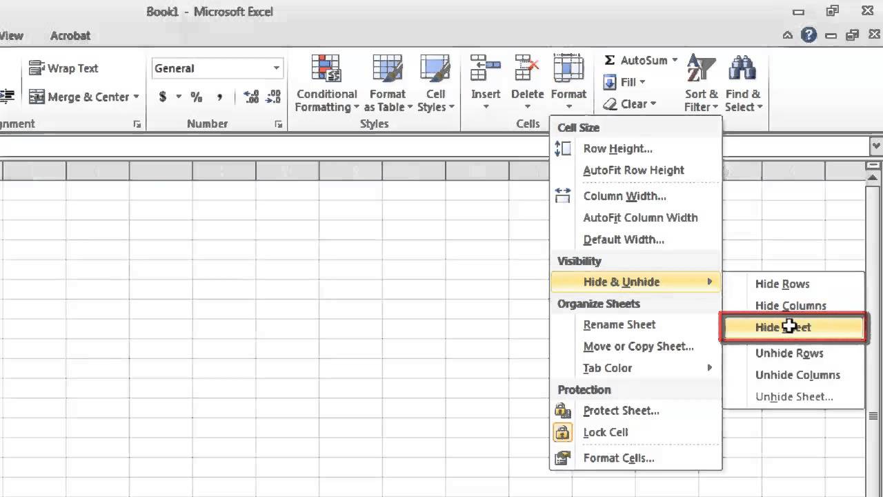
Using the Format Options in the Ribbon

The Ribbon in Excel offers another way to manage your spreadsheet’s layout:
- Select the rows adjacent to the hidden ones.
- Go to the Home tab on the Ribbon.
- Click on Format in the Cells group.
- Hover over Hide & Unhide and select Unhide Rows.
Using VBA for Automated Unhiding

For more advanced users or those looking to automate tasks, VBA can come in handy:
- Press Alt + F11 to open the VBA editor.
- Insert a new module by right-clicking on any open space in the left panel.
- Enter the following code:
| Code |
|---|
Sub UnhideAllRows()
    With ActiveSheet
      .Rows.Hidden = False
    End With
  End Sub
|

- Run the macro by pressing F5.
💻 Note: VBA automation can be a game-changer for repetitive tasks, but requires some learning.
Wrapping Up

Excel, as a powerful tool, gives you multiple avenues to manage your data. Knowing how to unhide rows in various ways ensures you’re never stuck, unable to access the information you need. Whether you prefer the quick shortcut, the visual cue of the context menu, or the precision of the Name Box, you’ve now got the know-how to make your work more efficient. Remember, mastering these techniques will not only save time but also help in keeping your work organized and accessible.
What’s the quickest method to unhide rows in Excel?

+
The fastest way to unhide rows in Excel is by using the keyboard shortcut Ctrl + Shift + 9. Select the rows around the hidden one(s) and press the shortcut to quickly reveal them.
Can I unhide multiple rows at once?

+
Yes, you can unhide multiple rows simultaneously by selecting the range of rows that includes the hidden ones, then right-clicking and selecting ‘Unhide’ or using the Ribbon’s ‘Unhide Rows’ option.
Why can’t I unhide some rows in Excel?

+
If rows appear to be unhidden but still aren’t visible, it’s possible that filters or grouping are applied to the sheet, making rows seem hidden. Check for filter icons or collapsed group markers and adjust accordingly to reveal all data.


