Merge Two Excel Sheets: Match and Combine by 2 Columns Easily

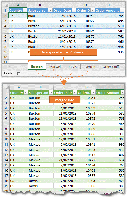
If you've ever had to deal with multiple Excel spreadsheets, you might have run into the challenge of combining data from two sheets into one cohesive dataset. This is especially pertinent when working with large volumes of data where manual merging would be impractical. In this comprehensive guide, we'll walk through several methods to merge two Excel sheets by matching and combining data from two columns. Whether you're using the latest version of Excel or working with the Microsoft 365 suite, we've got you covered.

Understanding the Basics

Before diving into the how-to, it’s beneficial to understand what merging Excel sheets entails. Essentially, you’ll be matching records from one sheet with another, based on criteria you define—typically one or more key columns. This merging can help eliminate duplicates, fill in missing data, or combine related information.

Key Concepts:

• Matching Criteria: These are columns you use to determine how records align between sheets.
• Unique Identifiers: Ideally, your sheets should have columns with unique identifiers like email addresses, employee IDs, or product codes.
• Combining Data: This is where you integrate data from matched rows into one comprehensive row.

Method 1: Using VLOOKUP

VLOOKUP (Vertical Lookup) is an Excel function commonly used for data merging. Here’s how to use it:

1. Open both Excel sheets: Ensure both files are in the same Excel workbook or one can reference another.
2. Choose your VLOOKUP column: Identify which column from sheet 1 you want to use to match with sheet 2. For example, if you're matching by 'Product ID' in both sheets, this becomes your lookup column.
3. Create a new column: In sheet 1, insert a new column where you'll pull data from sheet 2.
4. Enter the VLOOKUP formula: Use the formula structure:
   =VLOOKUP(A2, Sheet2!A:B, 2, FALSE)
   Here, A2 is the lookup value in sheet 1, 'Sheet2!A:B' is the table array from which to look up data, 2 specifies the return column, and FALSE means an exact match.

Method 2: Index Match

The Index Match function is often preferred over VLOOKUP due to its flexibility. Here’s the process:

1. Set up your sheets: Just like with VLOOKUP, ensure both sheets are accessible in your current workbook.
2. Create a new column: Add a column to sheet 1 for data retrieval from sheet 2.
3. Apply the formula: =INDEX(Sheet2!B:B,MATCH(A2,Sheet2!A:A,0))
   Here, A2 is the lookup value in sheet 1, Sheet2!A:A is the lookup array, and Sheet2!B:B is the column from which data is returned. The "0" argument specifies an exact match.

Notes:

🔍 Note: INDEX MATCH can be more powerful than VLOOKUP because it allows for searching to the left of the lookup column and can be combined with multiple criteria.

Method 3: Power Query (Get & Transform Data)

Power Query, available in Excel 2013 and later versions, provides a robust way to merge data:

1. Access Power Query: Go to Data > Get & Transform Data.
2. Load both sheets: Load both sheets into Power Query.
3. Merge Queries: Use the 'Merge Queries' feature. Choose your matching columns, set the join type (usually Left Outer), and preview the results.
4. Expand the merged column: Click on the expand arrow to include additional columns from the second sheet.
5. Load data: Once merged, you can load the new table into Excel.

Method 4: Using Excel Macros

For those comfortable with VBA, macros can automate merging:

1. Open the Visual Basic Editor: Press ALT + F11 or navigate to Developer > Visual Basic.
2. Write the VBA code: Below is an example macro that merges data based on two columns:

   Sub MergeSheets()
       Dim ws1 As Worksheet, ws2 As Worksheet
       Dim lRow As Long, i As Long
       Set ws1 = Worksheets("Sheet1")
       Set ws2 = Worksheets("Sheet2")
       lRow = ws1.Cells(ws1.Rows.Count, 1).End(xlUp).Row
       
       For i = 2 To lRow 'Assuming headers in row 1
           'Lookup value from ws1 to ws2 based on matching columns (A and B)
           On Error Resume Next
           ws1.Cells(i, 4).Value = Application.WorksheetFunction.VLookup(ws1.Cells(i, 1), _
                                                                         ws2.Range("A:B"), 2, False)
           On Error GoTo 0
       Next i
   End Sub
   
   

3. Run the Macro: After writing, save, close the editor, and run the macro from Excel.

Notes:

💡 Note: Macros can save a lot of time when you have to perform repetitive tasks but require some knowledge of VBA.

To sum up, merging two Excel sheets by matching and combining data from two columns is not just about convenience; it's about enhancing data integrity, reducing manual errors, and improving workflow efficiency. Whether you choose VLOOKUP for its simplicity, Index Match for flexibility, Power Query for advanced operations, or VBA macros for automation, each method offers unique advantages. With these techniques, you can efficiently integrate data from disparate sources, ensuring you have a comprehensive and accurate dataset ready for analysis.

Can I merge Excel sheets with different column headers?

+

Yes, you can. However, ensure that you match the columns manually or adjust your formulas to correctly reference the corresponding columns.

What if I need to merge based on multiple criteria?

+

Using Excel’s Index Match function or Power Query are more suitable for complex merges involving multiple criteria.

Are there any Excel features that simplify merging sheets?

+

Power Query in Excel 2016 and later versions provides a user-friendly interface to merge multiple sheets without needing to write formulas or code.