Match Items in Two Excel Sheets Easily

In today's data-driven business environment, managing and comparing large sets of data efficiently is crucial. Excel remains a powerful tool for such tasks, especially when it comes to matching data between two spreadsheets. Whether you're reconciling financial records, tracking inventory, or managing customer databases, being able to match items quickly and accurately can save hours of manual labor.

Understanding the Basics

Before diving into the methods of matching items, let’s clarify what matching means in this context:

• Matching: This involves comparing two lists to find records that are either identical or meet specific criteria. This could be a match based on an exact value, partial match, or even fuzzy logic where close matches are considered.
• Data Comparison: This goes beyond simple matching to look at differences, redundancies, or updates needed between two datasets.

Manual Matching vs. Automated Techniques

Manual matching involves looking through each row of both sheets manually, which is inefficient and prone to errors. Here’s where automated techniques come into play:

• VLOOKUP: This function allows you to search for a lookup value in one column and retrieve a value from the same row in another column. It’s effective for exact matches.
• INDEX/MATCH: Provides more flexibility than VLOOKUP, allowing for both vertical and horizontal lookups.
• Conditional Formatting: While not a matching function per se, it can highlight differences visually which can be useful for manual checks.

Step-by-Step Guide to Matching Items Using Excel

Using VLOOKUP for Simple Matches

Here’s how you can use VLOOKUP to match items:

1. Select the Cell: Choose the cell where you want the result of the VLOOKUP to appear.
2. Enter VLOOKUP Formula:

   =VLOOKUP(lookup_value, table_array, col_index_num, [range_lookup])

• lookup_value is the value you want to find in the first column of another table.
• table_array is the range of cells that contains the data.
• col_index_num specifies which column to return the value from.
• [range_lookup] (optional) - use FALSE for an exact match.
3. Drag Formula Down: Apply this formula to the entire column to match all entries.

Using INDEX/MATCH for More Flexible Matches

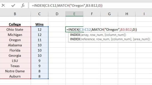
The INDEX/MATCH combination provides more versatility:

1. Identify Columns: Decide which columns in both sheets you will be matching on and which columns contain the data you want to return.
2. Enter INDEX/MATCH Formula:

   =INDEX(return_range, MATCH(lookup_value, lookup_range, 0))

• return_range is the array of cells from where the returned value will come.
• lookup_value is the value you want to find.
• lookup_range is the column or row where you are looking for the lookup_value.
• The last argument 0 in MATCH specifies an exact match.

🔍 Note: While VLOOKUP is simpler, INDEX/MATCH is more powerful because it can look in any direction, not just from left to right like VLOOKUP.

Advanced Techniques for Matching Data

Using Conditional Formatting

Although not a matching function, conditional formatting can help visualize matches or mismatches:

1. Select the range of cells you want to format.
2. Go to Home > Conditional Formatting > New Rule > Use a formula to determine which cells to format.
3. Enter a formula like =$A1<>B1 to highlight cells where values differ between columns A and B.

Power Query for Complex Matches

For those dealing with complex data matching scenarios, Power Query can be immensely helpful:

• Open Power Query from the Data tab, and load your tables into Query Editor.
• Use Merge Queries to match tables based on one or more common fields.
• Configure the type of join (Inner, Left, Right, Full) as per your matching needs.
• Expand the merged table to show the matched columns in your dataset.

💡 Note: Power Query can handle much more complex matching operations, including handling duplicates or transforming data before matching.

Common Pitfalls and Troubleshooting

• Data Format Inconsistency: Ensure the data types (numbers, dates, texts) match in both sheets before matching.
• Blank Spaces: Spaces can cause mismatches, especially with text-based lookups. Use TRIM() to remove leading or trailing spaces.
• Case Sensitivity: Excel’s standard lookup functions are not case-sensitive. For case-sensitive matching, use EXACT() function within array formulas or custom VBA.

Final Thoughts

Matching data between two Excel sheets is a fundamental skill that can significantly enhance your data management capabilities. Whether you’re reconciling accounts, verifying data integrity, or simply organizing information, Excel’s built-in functions like VLOOKUP, INDEX/MATCH, and the power of Power Query make this task much more manageable. Remember, the key to successful matching lies in understanding the nature of your data, ensuring its consistency, and choosing the right tools for the job. By implementing these strategies, you’ll find that what might have taken hours can now be accomplished in mere minutes, freeing up your time for more strategic tasks.

Can Excel handle case-sensitive matches?

+

Yes, but it requires additional functions or VBA to achieve this. The standard lookup functions like VLOOKUP are not case-sensitive.

What is the difference between VLOOKUP and INDEX/MATCH?

+

VLOOKUP can only look rightward from the lookup column while INDEX/MATCH can look in any direction. INDEX/MATCH is also more flexible with range adjustments and is less prone to errors when column orders change.

How can I avoid errors due to leading or trailing spaces?

+

Use the TRIM() function to remove spaces. Include it in your lookup or match formulas to clean the data before comparison.

Is there a limit to how much data Excel can handle for matching?

+

Yes, Excel has limitations based on the version, but with Power Query, you can manage much larger datasets by refreshing data from external sources like SQL Server.

Can Excel perform partial matches?

+

Yes, by using wildcards like * (asterisk) for any number of characters, or ? (question mark) for a single character in functions like VLOOKUP or MATCH.