Match Data in 2 Excel Sheets Effortlessly

Introduction

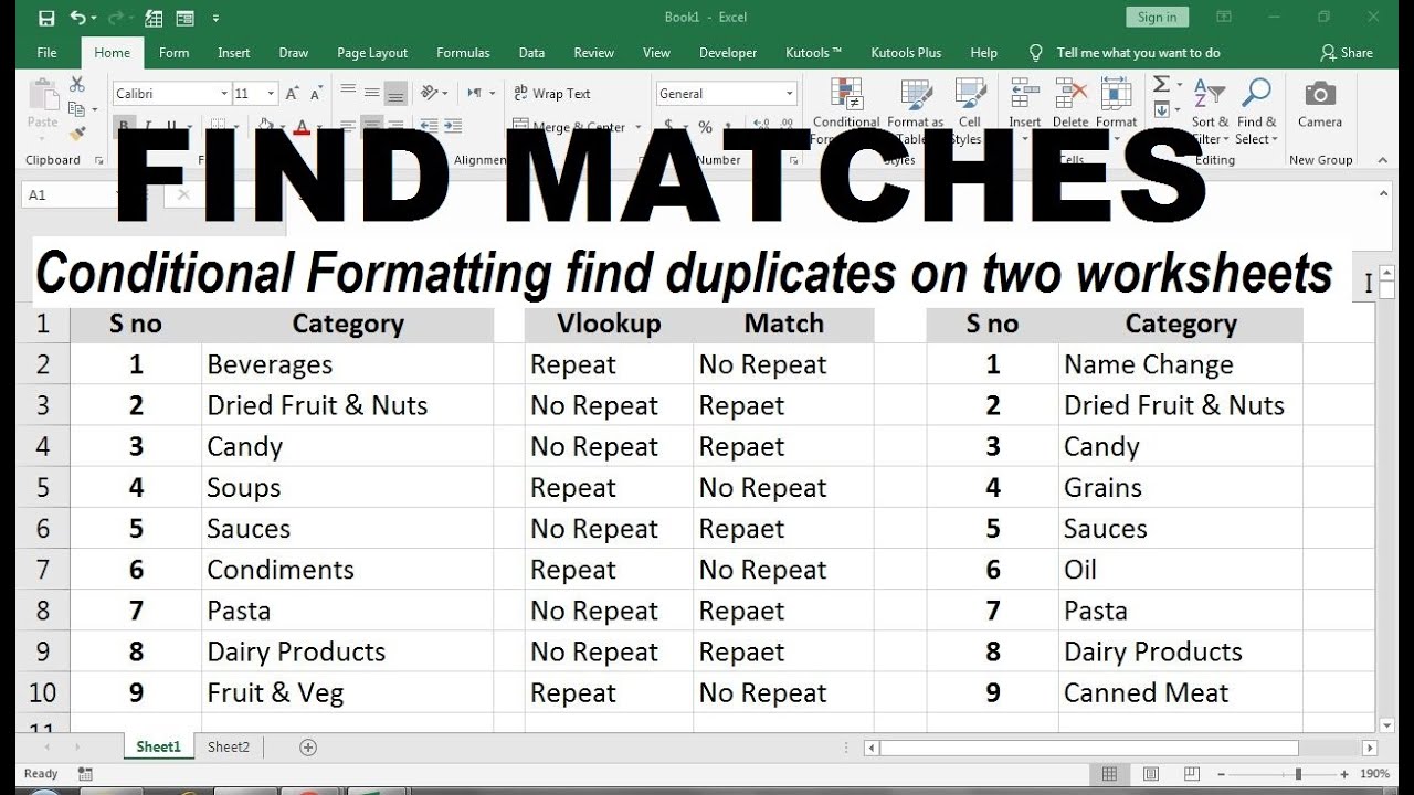
In today's data-driven business environment, efficiently handling and matching data between spreadsheets is critical. Excel, with its robust functions and user-friendly interface, remains a top choice for professionals to manage large sets of information. However, when dealing with two different Excel sheets, aligning and comparing data can be quite the challenge. This post will guide you through effective methods to match data in two Excel sheets, ensuring accuracy, saving time, and enhancing productivity.
The Challenge with Data Matching

Before diving into the solutions, it's essential to understand the common issues: - Data Inconsistency: Variations in data entry can lead to mismatches. This might occur due to different formats, spellings, or abbreviations. - Volume of Data: As datasets grow, manually checking and matching becomes impractical. - Structural Differences: Sheets might have different layouts, making direct comparison challenging. To address these challenges, we'll explore several techniques for data matching in Excel, optimizing for both simplicity and efficiency.
Methods for Matching Data

Excel offers multiple tools and functions to help compare and match data. Here’s a step-by-step guide:
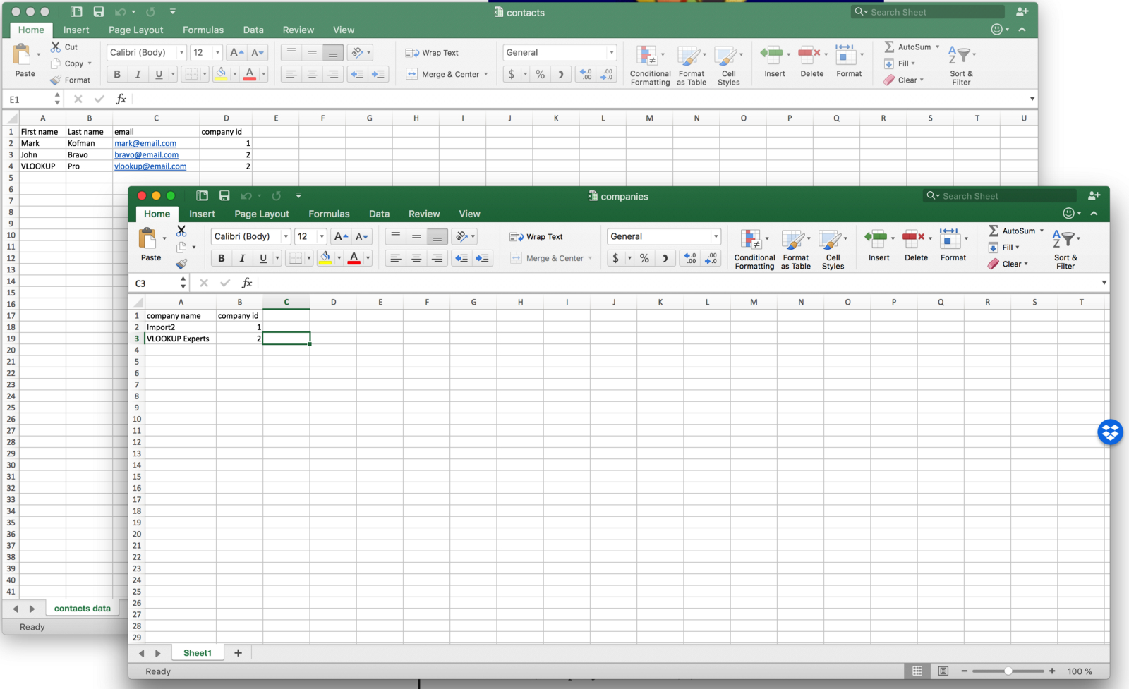
1. Using VLOOKUP or INDEX-MATCH

The VLOOKUP function, paired with INDEX-MATCH, is a staple for matching data:
- Open both Excel sheets.
- Identify the common field or key to match between the sheets.
- In the first sheet, enter the following formula to match values from the second sheet:
=VLOOKUP(A2,Sheet2!A$2:$B$100,2,FALSE)
📘 Note: Replace A2 with the cell containing your key in the first sheet, adjust Sheet2!A$2:$B$100 to reflect the range in the second sheet, and change 2 to the column number from which you want to retrieve the data. Use FALSE for an exact match.
If VLOOKUP isn't suitable due to data placement, INDEX-MATCH can be an alternative:
=INDEX(Sheet2!B$2:$B$100,MATCH(A2,Sheet2!A$2:$A$100,0))
📘 Note: In this formula, INDEX retrieves data, while MATCH finds the position of the key in Sheet2.
2. Conditional Formatting

Conditional formatting visually identifies matching or non-matching data:
- Select the range in Sheet1.
- Go to Home > Conditional Formatting > New Rule.
- Choose "Use a formula to determine which cells to format."
- Enter a formula like
=ISERROR(MATCH(A2,Sheet2!$A:$A,0))to highlight mismatches.
3. Using Advanced Filter

Advanced Filter can also help in matching data:
- Select the data range in Sheet1.
- Navigate to Data > Filter > Advanced Filter.
- Choose "Copy to another location" and select "Unique records only."
- Enter the criteria range from Sheet2 in the "List range" box.
- Specify a destination for the results.
4. Power Query

For advanced users, Power Query is a powerful tool:
- Go to Data > Get Data > From Other Sources > From Microsoft Query.
- Select the workbook and load the data from both sheets.
- Use the Merge Queries function to match data.
Creating a Table for Data Matching

| Excel Sheet 1 | Excel Sheet 2 |
|---|---|
| Key | Key |
| Value | Value |
| VLOOKUP Formula | Result |
=VLOOKUP(A2,Sheet2!A$2:$B$100,2,FALSE) |
Matched Value |

Key Points to Remember

When matching data:
- Always ensure the key field or unique identifier is present and consistent across both sheets.
- Be mindful of the formula limitations and data formats which can affect the matching process.
- Save frequently to avoid data loss.
In conclusion, Excel provides multiple avenues for effectively matching data between two sheets, ensuring accuracy and efficiency in your work. Whether you’re using traditional functions like VLOOKUP or exploring modern tools like Power Query, the method you choose will depend on the complexity of your dataset and your familiarity with Excel. By mastering these techniques, you’ll be able to enhance your workflow and make data comparison a seamless part of your data management tasks.
What is the difference between VLOOKUP and INDEX-MATCH?

+
VLOOKUP searches for a value in the first column of a table and returns a value in the same row from another column. INDEX-MATCH, on the other hand, is more flexible; it allows you to look up values both horizontally and vertically, making it less susceptible to structural changes in your data layout.
Can I use these methods for matching date-based data?

+
Yes, you can. Ensure that the date formats are consistent across both sheets. Excel functions like VLOOKUP and INDEX-MATCH can work with dates as long as they are treated as numeric values or properly formatted strings.
Are there any shortcuts or tips for large datasets?

+
For large datasets, using Power Query can significantly speed up the process. Additionally, converting your data into Excel tables can provide dynamic ranges for your formulas, making updates easier. Also, consider using CTRL + SHIFT + Enter to create array formulas for more complex matching operations.
How do I deal with duplicate keys?

+
Duplicate keys can complicate matching processes. Use Excel’s Advanced Filter to filter out duplicates or consider using functions like COUNTIF to count duplicates before matching. Also, Power Query can handle duplicates through the “Remove Duplicates” feature.


