5 Ways to Use VLOOKUP Between Excel Sheets

5 Ways to Use VLOOKUP Between Excel Sheets

If you've ever found yourself struggling to connect data across multiple Excel worksheets, then VLOOKUP is a tool that could change the way you work with spreadsheets forever. Here are five practical ways to harness the power of VLOOKUP to streamline your data analysis process across different sheets:

1. Basic VLOOKUP Across Sheets

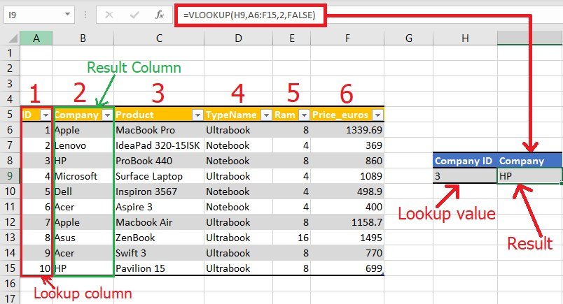
VLOOKUP is used to look up a value in the first column of a table and return a value from the same row in another column. Here's how to use it across sheets:

• Select the cell where you want to place the VLOOKUP result.
• Start with the formula =VLOOKUP(.
• The first argument should be the lookup value.
• Next, specify the range from another sheet (e.g., 'SheetName'!A:B).
• Define the column index number from which you want to retrieve the data.
• Decide whether you want an exact match by setting the range lookup argument to FALSE or an approximate match by using TRUE.

📝 Note: The lookup table must be in ascending order for an approximate match to work correctly.

2. VLOOKUP with Named Ranges

Named ranges make formulas easier to read and maintain:

• Define a named range for the data in your source sheet.
• In the target sheet, use VLOOKUP with the named range instead of cell references.
• Your formula will look something like =VLOOKUP(A1, NamedRange, 2, FALSE).

3. VLOOKUP for Data Consolidation

VLOOKUP can help consolidate data from multiple sheets:

• Create a summary sheet with categories or IDs you want to consolidate.
• Use VLOOKUP to pull data from multiple sheets into this summary sheet.
• Construct a formula that looks like this for each piece of data:=VLOOKUP(A2, 'Sheet2'!A:B, 2, FALSE), =VLOOKUP(A2, 'Sheet3'!A:B, 2, FALSE), etc.

💡 Note: This method helps visualize related data from various sources, enhancing data analysis.

4. Using VLOOKUP with CHOOSE Function for Vertical Data Retrieval

Combine VLOOKUP with CHOOSE to retrieve data from multiple columns:

• Use CHOOSE to create a virtual array from non-adjacent columns.
• Implement VLOOKUP on this array.

  =VLOOKUP(A2, CHOOSE({1,2}, Sheet1!A:A, Sheet2!B:B, Sheet3!C:C), 2, FALSE)
  

This technique allows you to look up data vertically across sheets without having to shift data around.

5. Dynamic VLOOKUP with Index-Match

To make your VLOOKUP more dynamic and flexible:

• Combine INDEX and MATCH functions to perform a lookup across different sheets.
• Instead of using VLOOKUP directly, use:

  =INDEX(Sheet2!B:B, MATCH(A2, Sheet2!A:A, 0))
  

• This method lets you handle dynamic ranges and is often more robust than VLOOKUP alone.

⚠️ Note: INDEX-MATCH can handle leftward lookups and is less prone to errors due to column shifts.

In conclusion, mastering VLOOKUP to work between Excel sheets enhances your data manipulation capabilities significantly. By implementing these five methods, you can efficiently manage large datasets, make data entry and analysis less tedious, and ultimately increase your productivity. Whether you're consolidating data, looking up values dynamically, or just trying to make your spreadsheets more manageable, these techniques provide a robust toolkit for any Excel user.

Can VLOOKUP look up values from different Excel files?

+

VLOOKUP can look up values from different sheets within the same Excel file. If you need to look up from different files, consider using External References or Power Query to combine files into a single workbook.

What if the sheet name changes in a VLOOKUP formula?

+

Use INDIRECT function with CONCATENATE or TEXTJOIN to dynamically reference the sheet name. This allows the VLOOKUP to adjust if the sheet name changes: =VLOOKUP(A2,INDIRECT(“‘”&B1&“’!A:B”),2,FALSE) where B1 contains the sheet name.

How do I prevent VLOOKUP errors?

+

Always check for exact matches by setting the last argument of VLOOKUP to FALSE, and use error handling functions like IFERROR to manage errors gracefully.