Effortless Excel: Compare Columns Across Sheets Easily

When working with large datasets in Excel, one of the common tasks is to compare data across different sheets. Whether you're tracking inventory, managing finances, or analyzing customer data, the ability to quickly identify differences and similarities can save countless hours. In this comprehensive guide, we'll delve into several methods for comparing columns across sheets in Excel, making the process not only efficient but also less error-prone.

Understanding the Basics of Sheet Comparison

Before we jump into the methods, let’s understand why comparing columns across sheets is necessary:

• Data Integrity: To ensure data consistency across various versions or sources.
• Error Checking: Spotting discrepancies that might indicate errors or require attention.
• Merge and Consolidate: Preparing for merging data from multiple sources into a single cohesive dataset.

Method 1: Using VLOOKUP to Compare Columns

VLOOKUP is one of Excel’s most versatile functions, and it can be adapted for comparing columns:

=VLOOKUP(A2, Sheet2!A:B, 2, FALSE)

Here’s how you can use it:

1. Select the column in the first sheet where you want to compare.
2. Enter the formula above in a new column, assuming your data starts from A2.
3. Sheet2!A:B refers to the sheet where you’re comparing against. Adjust this based on your sheet names.
4. The formula will return the corresponding value from the second column if there’s a match, or #N/A if there isn’t.

🔎 Note: VLOOKUP can be case-insensitive if not set to FALSE, which might lead to false positives in some scenarios.

Method 2: Conditional Formatting

Conditional formatting is an excellent visual tool for comparing columns:

1. Select the range you want to compare across sheets.
2. Go to Home > Conditional Formatting > New Rule.
3. Choose “Use a formula to determine which cells to format.”
4. Enter the following formula:

       =NOT(EXACT(A2, Sheet2!A2))
       

5. Set the desired formatting style.

This will highlight cells where there's a difference between the sheets, making discrepancies immediately visible.

Method 3: Using IF Function and ISERROR

Combining IF with VLOOKUP can give you more control over the output:

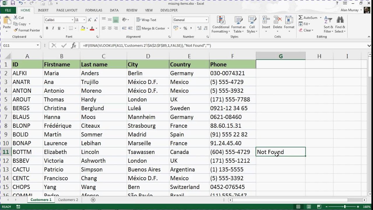
=IF(ISERROR(VLOOKUP(A2, Sheet2!A:B, 2, FALSE)), "Not Found", VLOOKUP(A2, Sheet2!A:B, 2, FALSE))

This method:

• Looks for the value in Sheet2.
• If not found, it displays "Not Found".
• If found, it returns the corresponding value.

Method 4: Advanced Filter

Excel's Advanced Filter can be used for a more dynamic comparison:

1. Copy both columns you want to compare into a new worksheet or a separate area of your current worksheet.
2. Use the Advanced Filter:
   • Go to Data > Advanced Filter.
   • Select "Filter the list, in-place" or "Copy to another location".
   • Choose the column from Sheet1 as the List range, and a similar range from Sheet2 as the Criteria range.

This method filters the data based on unique entries, highlighting items that are present in one sheet but not the other.

Comparing Multiple Columns Simultaneously

For a comprehensive comparison of multiple columns:

🔥 Note: You can also use COUNTIFS or SUMIFS functions for even more detailed comparisons across multiple sheets.

When to Use Each Method

Here’s a quick guide on when to use these methods:

• VLOOKUP: For straightforward matches or when you need to return a corresponding value from another column.
• Conditional Formatting: When you want a quick visual cue of discrepancies.
• IF/ISERROR: For when you need detailed control over the output (e.g., custom error messages).
• Advanced Filter: For comparing unique values across sheets.

Throughout this guide, we've highlighted various methods to compare columns across sheets in Excel. Each technique has its unique advantages, ensuring you can choose the best approach depending on the task at hand. Whether you're performing data validation, identifying discrepancies, or simply trying to make sense of large datasets, Excel offers powerful tools to simplify the process. Remember, the key to efficient data management lies not just in the tools but in understanding how to apply them effectively for your specific needs.

Can I compare more than two columns at a time?

+

Yes, Excel allows you to compare multiple columns using formulas or the Advanced Filter. However, the complexity increases with each additional column, so consider how best to structure your data for ease of comparison.

What should I do if VLOOKUP returns #N/A?

+

#N/A typically indicates that no match was found. You can use IFERROR or ISERROR functions to handle these cases gracefully or check for typos or data inconsistency across sheets.

How do I update the comparison dynamically as data changes?

+

Formulas like VLOOKUP and IF functions update automatically. For conditional formatting or filters, you might need to manually update the rules or apply them again.

Is it possible to compare columns with different data types?

+

Yes, but be cautious. Excel might treat numbers and text strings differently, which could lead to mismatches. Use conditional formatting or functions like TEXT or VALUE to ensure consistent data types for comparison.

What’s the best way to visualize these comparisons?

+

Conditional formatting offers an immediate visual cue. However, for large datasets, consider using charts like scatter plots, bar charts, or even conditional formatting heat maps to visually represent differences and similarities across sheets.