5 Easy Steps to Create Drop-Down Menus in Excel

Understanding Drop-Down Menus in Excel

Drop-down menus, or data validation lists, in Excel allow users to streamline data entry by restricting inputs to predefined options. This not only improves data consistency and accuracy but also enhances user experience by providing a more intuitive interface for entering data. In this blog post, we’ll dive into five straightforward steps to create these useful drop-down menus in your Excel spreadsheets.
Step 1: Planning Your Drop-Down Menu

Before you start creating a drop-down menu:
- Identify the cells or range of cells where you want the drop-down list to appear.
- Determine the source data for your drop-down items. This could be a list of names, categories, or any set of distinct values.
Plan your layout to ensure that the menu fits seamlessly into your worksheet’s design and purpose.
Step 2: Setting Up the Source Data

Source data is crucial for your drop-down menu:
- Select a column or row and enter all the options you want in the drop-down list.
- Ensure that there are no duplicates, and the list is clean. Here’s how it might look:
| Source Range |
|---|
| Apple |
| Banana |
| Cherry |

This data should be separate from where you’ll be applying the drop-down menu to avoid confusion.
🔍 Note: You can use dynamic ranges with Excel Tables or Named Ranges to make your source data more flexible.
Step 3: Applying Data Validation

To create the drop-down menu:
- Select the cell or cells where you want the drop-down menu.
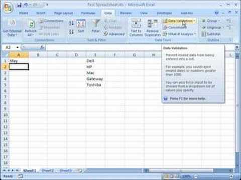
- Go to the Data tab, click Data Validation.
- In the Data Validation dialog:
- From the Allow: dropdown, select List.
- In the Source: field, either type the list entries separated by commas or refer to the range where you have listed your items.
Excel will now show a drop-down arrow when you click on any cell in the selected range.
Step 4: Customizing Your Drop-Down Menu

Excel provides several options to enhance your drop-down menu:
- Input Message: Add an explanatory message that appears when the cell is selected to guide users.
- Error Alert: Set up custom error messages for invalid entries, ensuring users stick to the list items.
These customizations can significantly improve the functionality and user-friendliness of your worksheet.
Step 5: Testing and Refining Your Drop-Down Menu

After setting up your drop-down menu:
- Test it by selecting various items to see if it works as expected.
- Check if the error alerts or input messages are appearing correctly.
- Ensure the menu does not obstruct data entry in adjacent cells.
This step is crucial for ensuring a seamless experience for all users.
By following these steps, you can effectively integrate drop-down menus into your Excel workbooks, enhancing both functionality and user interaction. Keep in mind that as your data changes or grows, you might need to adjust or expand your source data range. Remember to explore advanced techniques like using macros or VLOOKUP for more complex scenarios to make your drop-downs even more dynamic.
How do I make my drop-down list update automatically when the source data changes?

+
You can use Excel Tables or named ranges with dynamic formulas to ensure your list updates automatically. A table will expand or contract based on the data, and named ranges can use OFFSET or INDEX functions to define a dynamic range.
Can I create a dependent drop-down list where one list affects another?

+
Yes, you can! Use the INDIRECT function in data validation to create dependent lists. When a selection is made in the first drop-down, it changes the source of the second one.
What happens if a drop-down list cell is copy-pasted?

+
The drop-down menu will be copied, but the source data reference will not change unless it’s a relative reference or named range. Absolute references like “=A1:A5” will point to the same range in the new location, potentially causing errors if not adjusted.


