How to Freeze Excel 2013 Sheet Easily

Working with Microsoft Excel 2013 often involves managing large datasets that can easily become overwhelming, especially when you're dealing with extensive rows and columns. Freezing panes is a powerful feature that can make your life much easier by allowing you to keep parts of your sheet stationary while you scroll through the rest. Here, we'll explore how to freeze panes in Excel 2013, step by step, to help you master this useful tool for data management.
Why Freeze Panes in Excel 2013?

Before diving into the how-to, it’s beneficial to understand the “why” behind freezing panes. Here are a few reasons:
- Maintain Header Visibility: Keep row or column labels in view when scrolling through long datasets.
- Easier Navigation: Freeze panes can help you navigate through spreadsheets without losing context.
- Data Analysis: Comparing data becomes much more manageable when you can always see your reference points.
- Data Entry: Simplifies the process of entering data into specific fields or rows without losing track of column names or row numbers.
How to Freeze Panes in Excel 2013

1. Freeze the Top Row

If you need to keep the top row of your sheet visible:
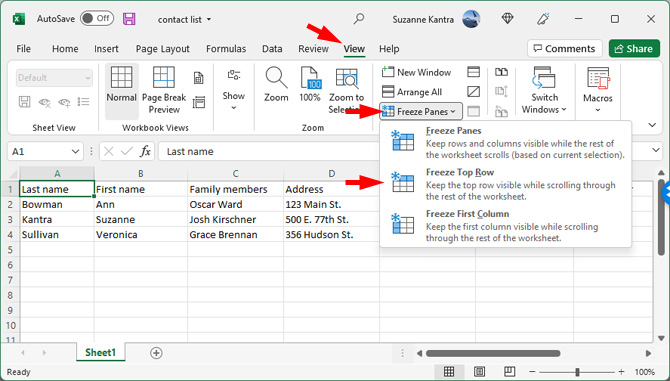
- Go to the View tab on the Ribbon.
- Locate the Window group.
- Click on Freeze Panes.
- Select Freeze Top Row from the dropdown menu.
🔖 Note: This will lock the first row so that it will remain on-screen even when you scroll down your sheet.
2. Freeze the First Column

For keeping the first column visible:
- Go to the View tab.
- Select Freeze Panes in the Window group.
- Choose Freeze First Column.
3. Freeze Multiple Rows or Columns

To freeze more than one row or column, follow these steps:
- Select the row below or the column to the right of where you want the split to appear.
- Go to the View tab.
- Click Freeze Panes and then choose Freeze Panes again.
- Excel will freeze all rows above the selected row and all columns to the left of the selected column.
4. Unfreeze Panes

If you decide you no longer need frozen panes:
- Go to the View tab.
- Click on Freeze Panes.
- Choose Unfreeze Panes.
It's worth noting that freezing panes can sometimes cause Excel to freeze or become unresponsive if you're working with very large datasets. This is due to the computational load Excel has to handle when rendering the frozen areas alongside scrollable content.
FAQ Section:

Can I freeze both rows and columns at the same time?

+
Yes, you can freeze both rows and columns simultaneously by selecting a cell where the rows and columns you want to freeze intersect. Then, choose ‘Freeze Panes’ from the View tab.
How do I know if my sheet has frozen panes?

+
You’ll notice a thin line separating the frozen panes from the rest of the worksheet. This line indicates where the freeze was applied.
Will freezing panes affect the data in my Excel sheet?

+
No, freezing panes doesn’t affect the data. It only changes the way you view and navigate the sheet, making it easier to work with large datasets without altering cell values or formulas.
In summary, freezing panes in Excel 2013 is a straightforward process that can significantly enhance your productivity when dealing with extensive spreadsheets. Whether you’re keeping important labels in view or comparing data across large areas, this feature ensures you never lose sight of your data’s context. Remember that while freezing panes can sometimes slow down performance with very large sheets, the convenience and functionality it offers make it a valuable tool for data management. Keep exploring Excel’s vast array of features to streamline your work even further!
This simple yet powerful feature of Excel can transform the way you work with data, making it more accessible and less time-consuming to manage complex spreadsheets.


