5 Ways to Spot Matching Numbers in Excel Sheets

Introduction
Discovering and matching numbers within large Excel sheets can often feel like searching for a needle in a haystack. However, with some handy techniques and Excel's powerful functions, you can streamline this process significantly. Whether you're reconciling financial data, consolidating reports, or just managing inventory, here are five robust methods to spot matching numbers in Excel sheets.
Method 1: Using Conditional Formatting

Conditional Formatting is one of Excel’s most visually appealing features, enabling users to quickly identify patterns and anomalies:
- Select the Range: Start by selecting the cells or range where you want to highlight duplicates.
- Go to Conditional Formatting: Navigate to the ‘Home’ tab, find the ‘Conditional Formatting’ option, and then click ‘New Rule.’
- Select Rule Type: In the ‘New Formatting Rule’ dialog, choose ‘Format only unique or duplicate values.’
- Specify Duplicates: From the dropdown, select ‘duplicate’ and choose a formatting style.
- Apply: Hit ‘OK’ to apply the rule.
🔹 Note: Make sure you are selecting the correct range to highlight; otherwise, you might miss some matching numbers.
Method 2: Using the VLOOKUP Function

The VLOOKUP function is excellent for cross-referencing numbers:
- Basic Formula: Use
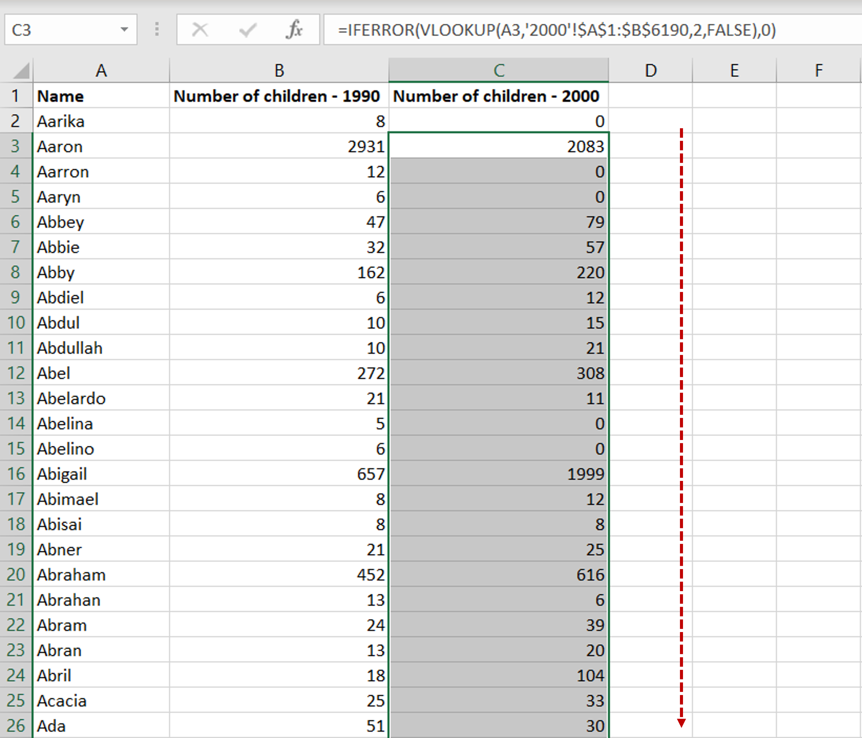
=VLOOKUP(lookup_value, table_array, col_index_num, [range_lookup]) - Example: Suppose you have two lists in cells A2:A10 and D2:D10. To find matching numbers, type
=VLOOKUP(A2, D$2$:D$10$, 1, FALSE)in cell B2 and drag it down. - Interpret Results: If the formula returns an error, the number in A2 does not exist in the range D2:D10.
Remember, when using VLOOKUP, ensure the data in both sheets is sorted in the same order for better performance.
Method 3: INDEX MATCH Combination

While VLOOKUP is straightforward, INDEX MATCH offers more flexibility:
- INDEX:
=INDEX(B1:B10, MATCH(A2, A1:A10, 0))returns the value in column B at the position where A2 matches in column A. - MATCH:
=MATCH(A2, A1:A10, 0)finds the position of A2 within the range A1:A10.
| Formula | Example |
|---|---|
| =INDEX(B:B, MATCH(A2, A:A, 0)) | Finds the value in column B corresponding to A2's position in column A. |

Method 4: Using COUNTIF Function

COUNTIF is excellent for finding duplicates based on frequency:
- Formula:
=COUNTIF(A:A, A2) - Example: In B2, you could enter
=COUNTIF(A:A, A2)and drag down. If the count is more than 1, the number appears multiple times. - Usage: This is particularly useful in large datasets where you want to know how many times a number repeats.
🔹 Note: Be cautious when using COUNTIF in very large datasets; it can be computationally intensive.
Method 5: Pivot Tables for Grouping and Counting

Pivot Tables are a powerful tool for analyzing data and finding matches:
- Create a Pivot Table: Select your data range, go to ‘Insert’ > ‘Pivot Table’.
- Set Up the Pivot Table: Drag the number field to both the ‘Row Labels’ and ‘Values’ areas. This will group the numbers and show counts.
- Identify Matches: Any number with a count greater than 1 is a match.
At this point, the transition to a wrap-up section feels natural, but let's maintain the flow to cover all methods.
To recap, using Excel to find matching numbers involves several approaches tailored to different user needs and data sets:
- Conditional Formatting: for visual identification.
- VLOOKUP and INDEX MATCH: for cross-referencing data.
- COUNTIF: to count occurrences of numbers.
- Pivot Tables: for a comprehensive analysis and visual grouping.
Each method has its merits, allowing users to select the most appropriate approach based on the complexity and size of the data they are working with.
What if my matching numbers are formatted differently?

+
To handle different number formats, you can use the TEXT function to standardize the format before searching for matches. For example, =TEXT(A2, "0") can convert all numbers to a standard text format for comparison.
Can I find matches for ranges of numbers, not just exact matches?

+
Yes, by using criteria within COUNTIFS or SUMIFS, you can find numbers that fall within specific ranges. For instance, =COUNTIFS(A:A, ">=" & 50, A:A, "<=" & 100) would count numbers between 50 and 100 inclusive.
How can I quickly highlight all unique values instead of duplicates?

+
Instead of selecting ‘duplicate’ in Conditional Formatting, choose ‘unique’ to highlight values that appear only once. This can be useful for identifying outliers or errors in your data.


