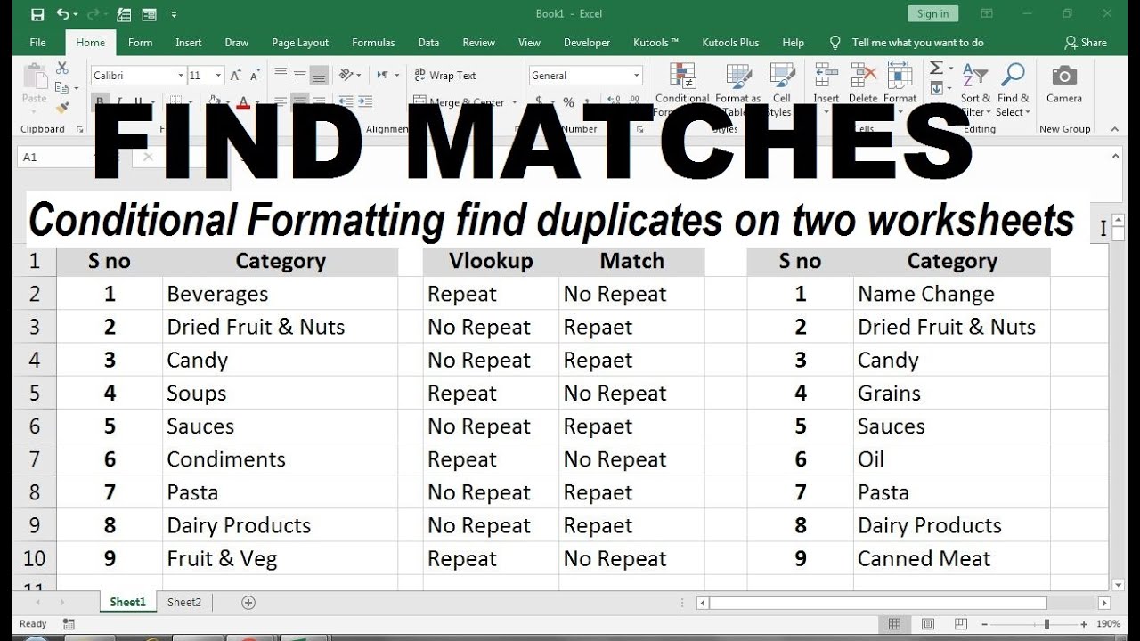
Find Matching Cells in Two Excel Sheets Easily

Do you often find yourself in a situation where you need to compare two Excel sheets to find matching cells? Whether you're reconciling financial data, merging databases, or simply trying to spot duplicates, Excel can be your friend with a few smart techniques. In this blog, we'll explore several methods to help you match cells in two different Excel sheets effortlessly.
Why Compare Excel Sheets?

Excel is a powerhouse for data manipulation, and there are numerous scenarios where comparing sheets becomes necessary:
- Quality Checks: Ensure data integrity by checking if entries match across sheets.
- Data Merging: Combine data from different sources to avoid duplication.
- Reporting: Identify discrepancies or matches for generating reports.
Method 1: Using VLOOKUP for Matching Cells

VLOOKUP, or Vertical Lookup, is one of Excel's most well-known functions for finding and retrieving data from a table:
- Select the cell in your second sheet where you want the matched data to appear.
- Enter the formula: ```excel =VLOOKUP(A2, Sheet1!A:B, 2, FALSE) ``` where A2 is the cell you want to match, Sheet1!A:B is the data range to look in, 2 is the column number containing the return value, and FALSE ensures an exact match.
- If there's a match, Excel will fill in the matching value from the specified column.
⚠️ Note: Ensure your lookup value is in the first column of the table range.
Method 2: Conditional Formatting for Visual Matching

If you need to see at a glance where cells match:
- Select the range in the first sheet.
- Go to Home > Conditional Formatting > New Rule.
- Choose “Use a formula to determine which cells to format."
- Enter this formula: ```excel =COUNTIF(Sheet2!A:A,A2)>0 ```
- Apply the format you want (e.g., background color).
Method 3: Advanced Filter to Find Matches

Advanced Filter can list all matches or only unique entries:
- Select the range you want to compare in the first sheet.
- Go to Data > Advanced under the Sort & Filter group.
- Check 'Copy to another location.'
- Define your criteria range in Sheet2, where you want the results.
- Use this formula: ```excel =Sheet1!A1:A50 ``` in your criteria range and click OK.
💡 Note: If you want to avoid duplicates, click 'Unique records only' in the Advanced Filter options.
Using Power Query for Match Finding

Power Query is an excellent tool for advanced data manipulation:
- Load both sheets into Power Query Editor.
- Merge Queries by choosing one key column in each sheet.
- Expand the matched columns for detailed comparison.
Scripting with VBA for Complex Matches

For those comfortable with programming, VBA (Visual Basic for Applications) allows for custom cell matching:
- Press Alt + F11 to open VBA editor.
- Insert a new module.
- Write your custom code to match cells based on your criteria.
👓 Note: VBA can automate repetitive tasks, but it requires some coding knowledge.
Excel is a versatile tool, and these methods for finding matching cells across sheets provide different levels of complexity and automation to suit your needs. Whether you're a beginner or an advanced user, there's a solution for you. Start with VLOOKUP for simple matching, use conditional formatting for visual aids, or delve into Power Query or VBA for more complex scenarios.
What if VLOOKUP can’t find a match?

+
If VLOOKUP returns #N/A, it means no exact match was found. Check for typos, formatting issues, or consider using INDEX-MATCH, which handles more dynamic data lookups.
Can I match cells across sheets with different column layouts?

+
Yes, especially with Power Query or VBA, which can align and compare columns regardless of their order.
Is there a way to match case-sensitive values in Excel?

+
VLOOKUP and other standard functions are not case-sensitive. However, you can use EXACT function in combination with IF to achieve this.


