5 Simple Steps for VLOOKUP Across Excel Sheets

Mastering VLOOKUP in Excel can transform how you manage data, especially when you need to pull information from various sheets. This guide outlines five simple steps to help you leverage VLOOKUP across different sheets effectively.
Step 1: Understand VLOOKUP

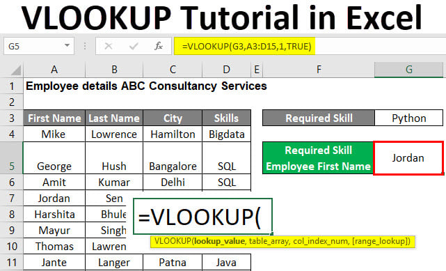
The VLOOKUP function in Excel searches for a value in the first column of a table and then returns a value from the same row in another column. Here’s its basic syntax:
- lookup_value: The value to search for in the first column.
- table_array: The range of cells that contains the lookup value.
- col_index_num: The column number from which to retrieve the value.
- [range_lookup]: Optional; TRUE for an approximate match or FALSE for an exact match.
Step 2: Prepare Your Sheets

Ensure that:
- Your sheets are clearly named.
- The lookup column is on the left-hand side in the source sheet.
- Data is consistent across sheets, including formatting and type.
📌 Note: For consistency, use the same format and naming convention across all related sheets to avoid confusion and errors.
Step 3: Use VLOOKUP Across Sheets

Follow these steps to perform VLOOKUP:
- Go to the cell where you want the result to appear in the destination sheet.
- Enter the VLOOKUP formula:
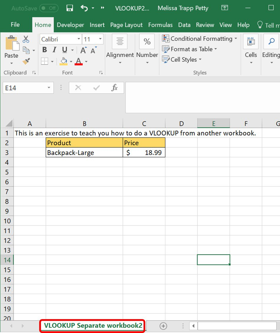
=VLOOKUP(lookup_value, ‘SheetName’!table_array, col_index_num, [range_lookup])Example: If you’re looking for “Product Code” in Sheet1 to retrieve the price from Sheet2:
=VLOOKUP(A2, Sheet2!A:B, 2, FALSE)🔍 Note: Ensure the column index number in your formula corresponds to the correct column in your source sheet.
Step 4: Handling Errors

Sometimes, VLOOKUP might return errors like #N/A or #REF! Here’s how to troubleshoot:
- Check for exact matches by setting the range_lookup argument to FALSE.
- Ensure the lookup_value exactly matches the data type in the source sheet.
- If the formula references an incorrect range, adjust it by modifying the table_array.
Step 5: Advanced Techniques

Enhance your VLOOKUP skills with these advanced techniques:
Combine with IFERROR

=IFERROR(VLOOKUP(lookup_value, ‘SheetName’!table_array, col_index_num, FALSE), “No Data”)This formula returns “No Data” instead of an error, improving the user experience.
Dynamic Sheet Reference

Use INDIRECT to refer to sheet names dynamically:
=VLOOKUP(A2, INDIRECT(“Sheet”&B2&“!A:B”), 2, FALSE)This allows you to lookup across sheets without changing the formula when sheet names change.
🖥️ Note: INDIRECT can slow down large workbooks, use it judiciously.
By following these steps, you've now learned how to efficiently use VLOOKUP across multiple Excel sheets. This technique will save time, reduce errors, and make data management more intuitive.
Can VLOOKUP pull data from multiple sheets at once?

+
While VLOOKUP itself does not pull data from multiple sheets simultaneously, you can nest VLOOKUPs within IF statements to achieve a similar result. Alternatively, use a combination of INDEX and MATCH functions for more complex scenarios.
What happens if the sheet name changes?

+
If you use direct references like ‘SheetName’, your formula will break if the sheet is renamed. Use dynamic sheet referencing techniques like INDIRECT to handle such changes automatically.
Is VLOOKUP case-sensitive?

+
No, VLOOKUP is not case-sensitive by default. If you need case sensitivity, you’ll need to combine it with other functions like EXACT or use VBA.
How can I make VLOOKUP search from right to left?

+
VLOOKUP can’t naturally search from right to left because it looks up values in the first column of the range. Use the combination of INDEX and MATCH functions to achieve this functionality.
What are the limitations of VLOOKUP?

+
Key limitations include:
- It only searches from left to right within its specified range.
- Performance can degrade with very large datasets.
- If you insert or delete columns within the lookup range, VLOOKUP formulas need to be updated to reflect these changes.


