Creating Excel Pivot Tables from Multiple Sheets Easily

If you're dealing with large datasets in Microsoft Excel, you'll find that Pivot Tables are incredibly powerful tools for summarizing, analyzing, and presenting your data effectively. But what if your data is spread across multiple sheets? Here's a comprehensive guide on how to create pivot tables from multiple sheets easily.
Why Use Pivot Tables?

Pivot Tables in Excel allow you to extract meaning from complex data arrays by providing:
- Dynamic Summarization: Quickly summarize, sort, count, and average your data.
- Data Exploration: Explore and drill down into your data to uncover insights.
- Flexible Reporting: Create reports that can be adjusted dynamically as data changes.
Steps to Create Pivot Tables from Multiple Sheets
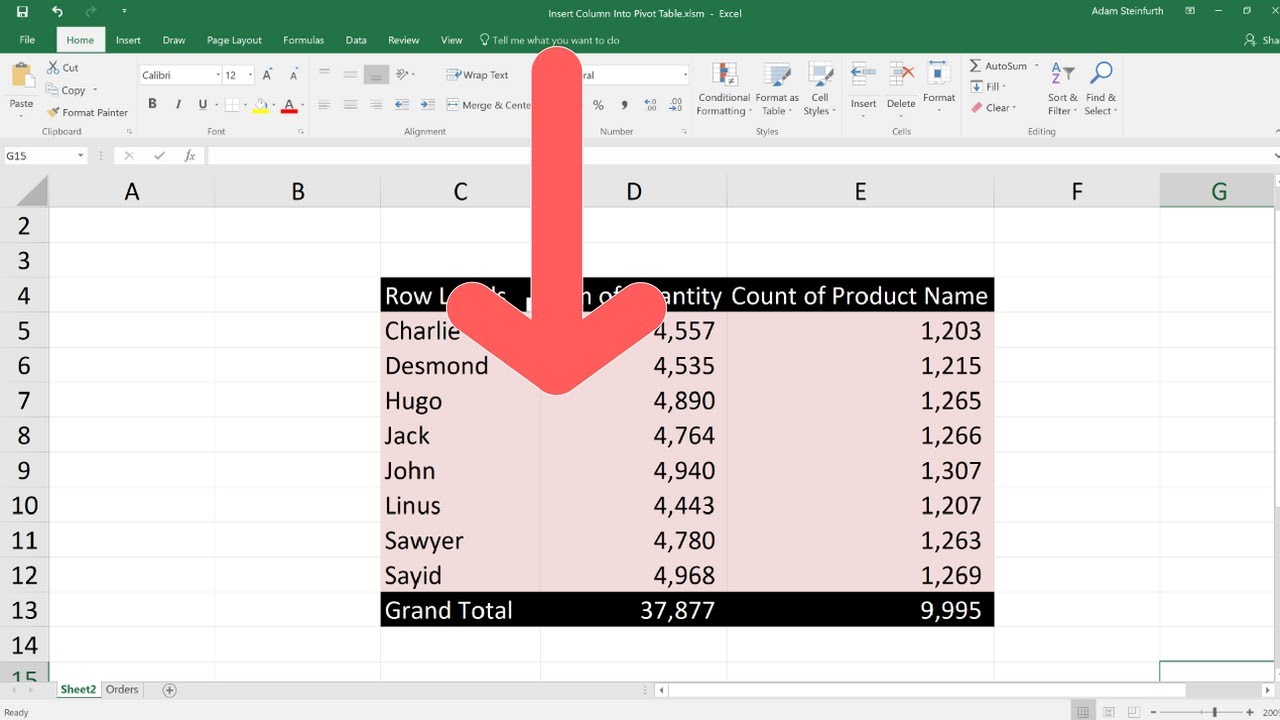
Here’s how you can leverage pivot tables from multiple sheets:
1. Prepare Your Data

Ensure that each sheet contains data in a consistent format. Here’s what you need to do:
- Make sure all datasets have the same columns in the same order.
- Name each sheet clearly to help with reference later.
- Ensure no merged cells or blank rows in your data range.
2. Add Your Data to a Query

Excel’s Power Query tool will be your friend here:
- Navigate to the Data tab and click on Get Data > From Other Sources > Blank Query.
- In the Power Query Editor, select Combine > Append Queries > Append Queries as New.
- In the “Append” dialog, choose each sheet you want to combine:
- Click Add >> to add sheets.
- Click OK when done.
⚠️ Note: Power Query is only available in Excel 2016 Professional Plus and Office 365 ProPlus.
3. Load Data into Excel

Once your data is combined:
- Click Close & Load to insert the query results into a new worksheet.
4. Create Your Pivot Table
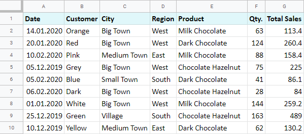
With the combined dataset ready:
- Select any cell within your new table.
- Go to the Insert tab and click on Pivot Table.
- Choose where to place your pivot table (New Worksheet or Existing Worksheet).
- In the Pivot Table Fields pane, drag fields to Rows, Columns, Values, and Filters as needed.
🔍 Note: Your pivot table will now dynamically reflect changes in the source data, allowing for real-time analysis.
Advanced Techniques

To enhance your pivot table:
- Use Slicers: Add slicers to filter your pivot table data visually.
- Create Calculated Fields: Insert formulas within your pivot table for custom calculations.
- Refresh Data: Remember to refresh your pivot table if the source data changes.
| Shortcut | Action |
|---|---|
| Alt + N, V | Opens the Insert Pivot Table dialog box |
| Alt + D, P | Alternative way to insert a Pivot Table |

📝 Note: When dealing with large datasets, ensure your Excel file is not too large to handle by Power Query.
In conclusion, creating pivot tables from multiple sheets can streamline your data analysis, providing insights that might have been overlooked in a fragmented data environment. By following these steps, you can harness the full potential of Excel's analytical tools to make informed decisions based on comprehensive data aggregation.
Can I create a pivot table if my data is in different workbooks?

+
Yes, you can, but you would need to consolidate all your data into one workbook first. Use the “Combine Queries” feature in Power Query to pull data from multiple workbooks.
What if my sheets have different column headings?

+
You’ll need to standardize the column headings across all sheets before creating the pivot table. This might involve manually renaming or aligning the columns to match.
How do I update my pivot table when data changes?

+
Right-click on the pivot table and select Refresh, or use the keyboard shortcut Alt + F5. This ensures your pivot table reflects the most current data.
Can I automate this process?

+
Yes, by using VBA scripts, you can automate the consolidation of data from multiple sheets and then create pivot tables automatically. This requires some programming knowledge.
