5 Simple Steps to Multiply Numbers in Excel Easily

Excel is not just a tool for crunching numbers but a versatile application that can streamline various data manipulation tasks, including multiplication. For those who work with financial data, analysts, or anyone dealing with quantitative information, understanding how to multiply in Excel is invaluable. This guide will walk you through 5 simple steps to perform multiplication in Microsoft Excel effortlessly, enhancing your productivity and accuracy in handling calculations.
Understanding the Basics

Before diving into the steps, let’s briefly discuss what multiplication in Excel entails. Excel uses standard mathematical operations, where the asterisk (*) symbolizes multiplication. Here’s what you need to know:
- Excel uses a straightforward formula syntax:
=number1*number2. - You can multiply numbers, cell references, or even entire columns or rows.
- The result of a multiplication is displayed in the cell where the formula is entered.

Step 1: Select the Cell for the Result

First, decide where you want the multiplication result to appear. Click on the cell where you wish to insert the formula.
- This cell will automatically adjust based on any changes made to the source cells, providing dynamic results.
- If you’re planning to use the result in other calculations, consider placing it in a convenient location.

Step 2: Enter the Multiplication Formula

In the formula bar or directly in the selected cell, type the formula for multiplication:
=number1*number2Here:
number1andnumber2can be either numerical values or cell references.- If using cell references, enter something like
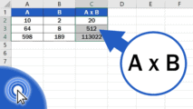
=A1B1where A1 and B1 contain the numbers to multiply.
📝 Note: Ensure there is no space between the asterisk () and the cell references or numbers.

Step 3: Complete the Formula and Press Enter

After entering your formula, press Enter. Excel will calculate the result and display it in your selected cell.
Key points to remember:
- The formula will update if the values in the referenced cells change.
- Excel has a built-in formula checker for syntax errors, which is helpful in ensuring accuracy.

Step 4: Formatting the Result

If necessary, you might want to format the result:
- Right-click on the cell containing the result, choose ‘Format Cells.’
- Select the desired number format, such as number, currency, or percentage.
- Adjust decimal places if required.
| Formatting Option | Description |
|---|---|
| Number | Displays numbers without any special formatting. |
| Currency | Adds the currency symbol and optional decimal places. |
| Percentage | Multiplies the number by 100 and adds a percent symbol. |

🖼️ Note: Proper formatting ensures clarity, especially when dealing with financial data or reports.
Step 5: Copying the Formula

If you need to multiply multiple values across rows or columns:
- Click on the cell with the formula.
- Hover your mouse over the bottom-right corner of the cell until you see a plus sign.
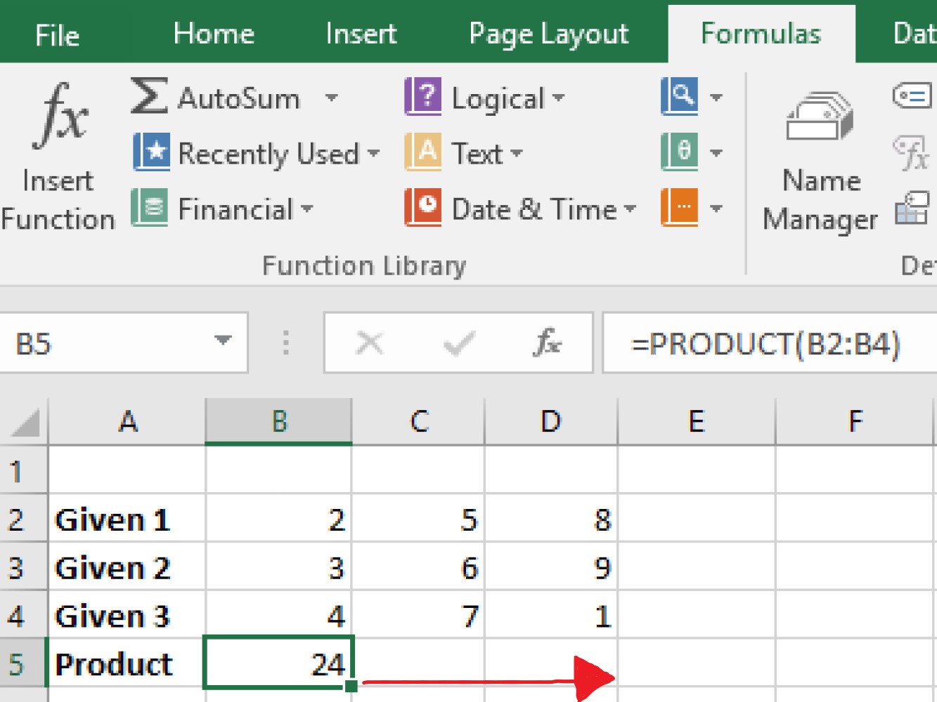
- Drag down or across to copy the formula to other cells, ensuring relative references adjust accordingly.
This method saves time and helps in maintaining consistency in calculations.
⏲️ Note: Excel’s auto-fill feature can be a lifesaver for repetitive tasks.
By following these 5 simple steps, you can easily multiply numbers in Excel, whether you're dealing with financial models, inventory management, or any other data-related task. Excel's ability to handle mathematical operations makes it an indispensable tool for data analysis, providing accuracy, speed, and flexibility in your work. As you become more familiar with these operations, you'll find that Excel offers a vast array of functions to explore, enhancing your ability to manage complex calculations with ease.
How do I multiply more than two numbers in Excel?

+
To multiply more than two numbers in Excel, simply extend the formula by adding additional asterisks and numbers or cell references. For example, =A1*B1*C1*D1 would multiply the values in cells A1, B1, C1, and D1.
Can I multiply entire columns or rows?

+
Yes, you can multiply entire columns or rows by using a formula in one cell and then dragging the formula across the cells you want to cover. Excel will adjust the cell references accordingly.
What if I want to multiply numbers and then sum the results?

+
You can use the PRODUCT function combined with SUM. For example, =SUM(PRODUCT(A1:A5,B1:B5)) will multiply A1 with B1, A2 with B2, and so on, then sum the results.
How can I handle errors in Excel calculations?

+
Excel provides several functions like IFERROR, ISERROR, and ERROR.TYPE to handle and identify errors in calculations, allowing you to either skip erroneous cells or display custom messages.


