Comparing Excel Sheets: Simplified Guide Using VLOOKUP

In the digital age, Microsoft Excel remains one of the most powerful tools for data manipulation and analysis. One common task that users often face is comparing data across different sheets within Excel. This task can range from simple to complex depending on the volume of data, its structure, and the level of detail needed in comparison. Here, we'll explore how to effectively compare Excel sheets using the VLOOKUP function, a versatile tool designed for looking up values in a table or a range.

Understanding VLOOKUP

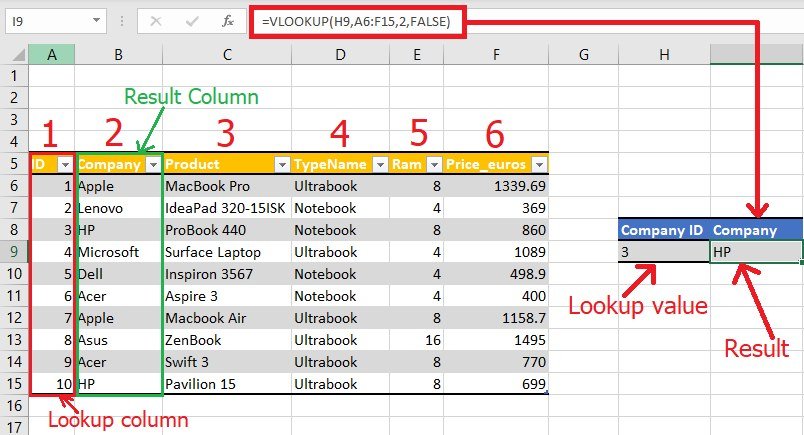
VLOOKUP stands for ‘Vertical Lookup.’ It searches for a value in the first column of a table and returns a value in the same row from another column. The basic syntax of VLOOKUP is:

VLOOKUP(lookup_value, table_array, col_index_num, [range_lookup])

• lookup_value: The value to search for in the first column of the table.
• table_array: The range of cells that contains the data.
• col_index_num: The column number in the table from which to retrieve the value.
• range_lookup: TRUE for an approximate match or FALSE for an exact match.

Steps to Compare Two Excel Sheets

To compare sheets, let’s assume we have two sheets, ‘Sheet1’ and ‘Sheet2’, both with a common identifier like employee ID:

Step 1: Setting Up Your Data

First, ensure your data in both sheets are similarly formatted:

• Columns in both sheets should align (e.g., Employee ID, Name, Department, etc.)
• The column containing the lookup value should be the same in both sheets

Step 2: Applying VLOOKUP

Here’s how to use VLOOKUP for comparing data:

1. Open the sheet where you want to compare data (let’s call it ‘Sheet1’).
2. In the cell next to your data, enter the following VLOOKUP formula:

=IF(ISNA(VLOOKUP(A2, Sheet2!A:B, 2, FALSE)), “Not Found”, VLOOKUP(A2, Sheet2!A:B, 2, FALSE))

• A2: This is the lookup value in Sheet1, corresponding to the employee ID or other identifier.
• Sheet2!A:B: This represents the table array from Sheet2, where column A contains the ID, and column B might contain names or other data for comparison.
• 2: The column number in Sheet2 from which you want to retrieve data. Adjust this number based on your data arrangement.
• FALSE: Specifies an exact match.
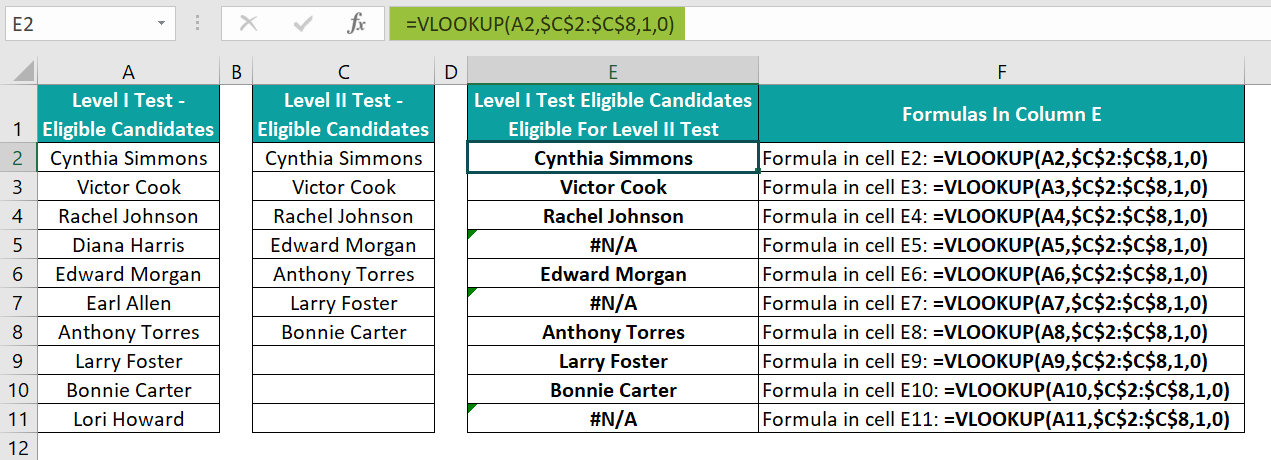
• IF/ISNA: This combination checks if the result from VLOOKUP is #N/A, meaning the data was not found.
3. Drag the formula down through the column to apply to all rows.

Step 3: Handling Mismatches and Additional Insights

After running VLOOKUP, you might want to:

• Highlight or color code mismatches for visual cues.
• Use Conditional Formatting to highlight cells where values do not match.
• Create a separate column for insights, like percentage changes or differences.

💡 Note: VLOOKUP can be time-consuming with large datasets. Consider using INDEX/MATCH or XLOOKUP in newer Excel versions for better performance.

Step 4: Advanced VLOOKUP Scenarios

Sometimes, the data structure might require more complex VLOOKUP usage:

Multiple Return Values

If you need to retrieve multiple values from the same row:

• Use multiple VLOOKUPs with different col_index_num values.

Wildcard Searches

If you’re matching patterns or parts of text:

• Add wildcards (*, ?) to your lookup_value to search for partial matches.

Handling Errors

Manage VLOOKUP errors effectively:

• Utilize IFERROR or IF(ISNA) to control how Excel handles lookup failures.

Wrapping Up

Comparing Excel sheets with VLOOKUP provides a straightforward way to analyze and contrast data between different datasets. This method is especially useful for tasks involving employee lists, inventory checks, or any situation where matching identifiers are involved. By mastering VLOOKUP, you can efficiently pinpoint differences or confirm similarities, enabling better decision-making with data at your fingertips. Remember, while VLOOKUP can handle many scenarios, for very large datasets or more advanced comparisons, exploring alternatives like INDEX/MATCH or Power Query might offer additional benefits.

What if my data doesn’t have a common identifier?

+

Use other functions like INDEX/MATCH, or consider concatenating multiple columns to create a unique identifier.

Can VLOOKUP compare multiple columns at once?

+

Not directly. You’d need to run multiple VLOOKUP functions or use an array formula or Power Query to accomplish this task.

Why might VLOOKUP return #N/A?

+

Common reasons include no match found, data type mismatch (e.g., text vs. number), or an incorrectly specified table array.

Is there a limit to the number of rows VLOOKUP can handle?

+

VLOOKUP doesn’t have an explicit row limit, but performance might degrade with very large datasets.