5 Ways to Vlookup Between Sheets in Excel Easily

Mastering the art of looking up data across multiple sheets in Microsoft Excel can significantly streamline your data management tasks. Whether you're managing financial statements, inventory lists, or any dataset that requires seamless data retrieval from different sheets, VLOOKUP is your go-to function. Here's a detailed guide on five effective ways to VLOOKUP between sheets in Excel.
1. VLOOKUP with Absolute Cell References

One of the simplest methods to VLOOKUP data between sheets is by using absolute cell references. This ensures that your lookup range remains constant even when you copy and paste the formula:
- Enter your VLOOKUP formula on the sheet where you want to pull the data.
- Instead of pointing directly to a cell range on another sheet, use the absolute reference (e.g.,
Sheet2!A1:B100).
=VLOOKUP(A1, Sheet2!A1:B100, 2, FALSE)
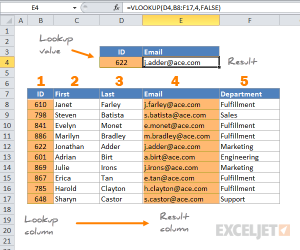
This formula searches for the value in A1 within the first column of the range on Sheet2 and returns the corresponding value from the second column.
🔍 Note: Absolute references ($ signs) keep the row and column from changing when copying the formula. This is crucial for maintaining consistency in your VLOOKUP lookups.
2. Indirect Function with VLOOKUP

For a more dynamic approach, combine VLOOKUP with the INDIRECT function. This method allows you to reference different sheets dynamically:
- Create a cell that contains the name of the sheet you want to reference.
- Use INDIRECT in your VLOOKUP formula to point to this cell:
=VLOOKUP(A1, INDIRECT(“‘” & A1 & “’!A1:B100”), 2, FALSE)
Here, if cell A1 on your current sheet contains “Sheet2,” the formula will effectively reference Sheet2!A1:B100.
3. Named Ranges

Named ranges provide a clean and reusable way to manage complex formulas:
- Define a named range for the lookup table on each sheet.
- Use the named range in your VLOOKUP formula:
=VLOOKUP(A1, MyRange, 2, FALSE)
‘MyRange’ could be a named range defined as Sheet2!A1:B100, making your formulas easier to read and maintain.
4. Data Consolidation

If your sheets share a common identifier, you might consider data consolidation:
- Create a consolidated sheet using Excel’s built-in consolidation tools or manually gather data.
- VLOOKUP within this consolidated sheet:
=VLOOKUP(A1, ConsolidatedSheet!A1:C1000, 2, FALSE)
This technique can simplify lookup when working with multiple sheets that need to be integrated into one view.
5. Excel Tables

Excel tables (introduced in Excel 2007) automatically expand when new data is added, making them ideal for VLOOKUP across sheets:
- Convert your data into an Excel table on each sheet.
- Use structured references in your VLOOKUP:
=VLOOKUP(A1, Sheet2!Data[ItemID], 2, FALSE)
Here, Data[ItemID] refers to the ItemID column in the table named “Data” on Sheet2.
By employing these methods, you can efficiently and accurately VLOOKUP data across multiple Excel sheets, enhancing your data management capabilities. Each approach has its advantages, and choosing the right one depends on the structure of your data and the specific tasks you need to accomplish.
What is the benefit of using absolute references in VLOOKUP?

+
Using absolute references ensures that your formula always looks in the same range of cells, which is crucial when you copy the formula across cells.
Can VLOOKUP look up data from another workbook?

+
Yes, you can reference data in another workbook by including the workbook's name in the formula, like =VLOOKUP(A1, '[OtherWorkbook.xlsx]Sheet1'!$A$1:$B$100, 2, FALSE). However, both workbooks must be open for the formula to work correctly.
How do you handle errors from VLOOKUP?

+
To manage VLOOKUP errors, you can use functions like IFERROR or ISERROR combined with VLOOKUP to handle cases where data is not found or there are other errors in calculation.
With these strategies, your Excel workflow becomes more fluid, your data management more efficient, and your analytics more insightful. Each method has its place, and understanding when to apply them can transform how you work with data in Excel.


