5 Ways to Reference Excel Sheets Easily

In the modern workplace, Excel is synonymous with efficiency and data management. Whether you're an accountant, a project manager, or an enthusiastic data analyst, knowing how to navigate through Excel sheets seamlessly can drastically boost your productivity. This article will delve into five practical methods to reference Excel sheets effortlessly, saving time and minimizing errors.
Method 1: Using the INDIRECT Function

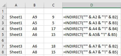
Excel’s INDIRECT function is a powerful tool that allows you to create a cell reference from a text string. Here’s how to use it effectively:
- Start with your source sheet, e.g., ‘Data’
- Enter the reference in another cell, e.g., A1: “=‘Data’!A1”
- Now, in the target sheet, use the formula
=INDIRECT(A1). This will automatically pull data from the cell referenced in A1 of the ‘Data’ sheet.
🔍 Note: The INDIRECT function updates automatically if the source sheet is renamed or if you change the cell reference in A1. Be cautious; if you move or delete sheets, the references will break.
Method 2: VLOOKUP Across Sheets

When data is spread across multiple sheets, using VLOOKUP can help connect these sources effectively:
- Identify the lookup value in the sheet you’re working on.
- Use
=VLOOKUP(lookup_value, ‘SheetName’!table_array, col_index_num, [range_lookup])where ‘SheetName’ is the name of the sheet containing your lookup table. - Ensure that the table array in the sheet you’re referencing is correctly formatted for VLOOKUP.
| Function Component | Description |
|---|---|
| lookup_value | The value you’re searching for |
| table_array | The range containing the lookup table |
| col_index_num | The column index from which to retrieve the result |
| range_lookup | TRUE for approximate match; FALSE for exact match |

Method 3: Named Ranges for Quick References

Named Ranges can significantly simplify your Excel formulas:
- Go to the Formulas tab > Define Name.
- Name your range, e.g., ‘SalesTable’.
- Now you can reference this range from any sheet using the name, like
’=SUM(SalesTable)for summing all data in that range.
🔎 Note: Named ranges can be scoped to the entire workbook or specific sheets. Consider this when defining names for avoiding conflicts.
Method 4: Using 3D References for Consistent Formulas

3D references let you work with the same range across multiple sheets:
- Select the first sheet where you want to apply the 3D reference.
- Hold down Shift, click on the last sheet in the series, then select your range.
- Use the formula:
=SUM(Sheet1:Sheet3!A1)to sum cell A1 across Sheet1, Sheet2, and Sheet3.
Method 5: Excel’s Lookup Wizard (for Advanced Users)

For those who thrive on Excel’s advanced features, the Lookup Wizard can be a game-changer:
- Use the VLOOKUP, HLOOKUP, or LOOKUP wizard found in the Formulas tab.
- Define your lookup range, and the wizard will help you craft the formula, reducing errors in sheet referencing.
🗝️ Note: The Lookup Wizard is available in Excel for Microsoft 365, but the steps might differ in older versions.
Understanding these five methods to reference Excel sheets can enhance your spreadsheet management capabilities, making complex data interaction look simple. These techniques not only streamline data manipulation but also help in ensuring accuracy across multiple sheets. By embracing these Excel functionalities, you can elevate your work efficiency and data analysis to professional levels.
What is the purpose of using INDIRECT function?

+
The INDIRECT function allows you to create a cell reference from a text string, making it ideal for creating dynamic links that update automatically when sheet names or references change.
How can 3D references improve my work?

+
3D references enable you to perform calculations across multiple sheets without having to adjust the formula, reducing complexity and errors in larger workbooks.
Why should I use Named Ranges?

+
Named Ranges make your formulas easier to read, maintain, and update, especially when your workbook contains numerous sheets or complex formulas.


