5 Simple Steps to Master VLOOKUP in Excel

Mastering VLOOKUP in Excel can dramatically increase your data analysis efficiency. Whether you're managing a business inventory or analyzing marketing data, VLOOKUP is an indispensable tool for searching and retrieving data from an Excel worksheet. Here are five simple steps to get you started:
Understanding VLOOKUP

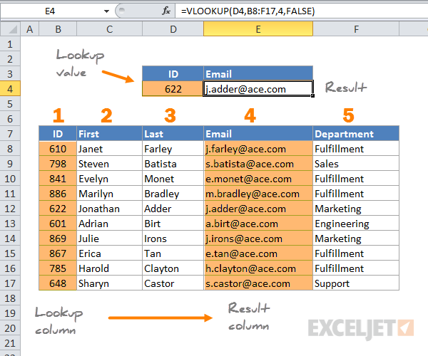
VLOOKUP, or Vertical Lookup, is a function that searches for a value in the first column of a table and returns a value in the same row from another column. Here's how it's structured:
- Lookup_value: The value you're searching for.
- Table_array: The range of cells that contain the data.
- Col_index_num: The column number from which to retrieve the value.
- Range_lookup: True for approximate match, False for an exact match.

Step 1: Prepare Your Data

Before you begin, ensure your data:
- Is organized in a vertical column format.
- Does not contain merged cells in the lookup column.
- Has no errors or spaces that might confuse Excel.
❗ Note: Avoid using VLOOKUP on data with variable structures as it may lead to errors or incorrect returns.
Step 2: Use VLOOKUP

Here's how you apply the function:
- Select the cell where you want the result to appear.
- Go to Formulas > Insert Function, search for "VLOOKUP", and click OK.
- Enter the lookup_value from your worksheet.
- Select the table_array by highlighting the necessary range.
- Enter the col_index_num which specifies the column to return from the table.
- Set range_lookup to True or False as needed.
Your VLOOKUP function might look like this:
=VLOOKUP(B2,A1:E100,3,FALSE)
Step 3: Handle Errors

VLOOKUP can return errors if it doesn't find a match:
- #N/A: If no exact match is found.
- #REF!: If the
col_index_numis greater than the number of columns in thetable_array. - #VALUE!: If
col_index_numis less than 1 or text/number format mismatch.
Use the IFERROR function to handle these errors:
=IFERROR(VLOOKUP(B2,A1:E100,3,FALSE),"Not found")
❗ Note: Using IFERROR with VLOOKUP provides a clean way to manage errors and maintain the integrity of your data analysis.
Step 4: Mastering Advanced Techniques

To take your VLOOKUP skills to the next level:
- Combine with other functions: Use VLOOKUP alongside CONCATENATE, LEFT, RIGHT, etc., to refine your lookups.
- Dynamic ranges: Utilize NAMED RANGES or Tables for more dynamic and flexible lookups.
- Array VLOOKUPs: For advanced users, consider using arrays with VLOOKUP to return multiple values at once.
Step 5: Practice

The best way to master VLOOKUP is through practical application:
- Create sample data sets to practice different lookup scenarios.
- Use VLOOKUP in real-world scenarios where data merging, searching, or updating is required.
| Scenario | VLOOKUP Usage |
|---|---|
| Employee Database | Retrieve employee contact information based on their ID. |
| Sales Report | Match product IDs to their respective sales totals. |

By following these steps, you can make VLOOKUP a fundamental part of your Excel toolkit. Remember, mastering any Excel function, including VLOOKUP, requires practice, and adapting these steps to real-world data will enhance your skills in data manipulation and analysis.
What does the “Col_index_num” parameter mean in VLOOKUP?

+
The Col_index_num refers to the column number in the table array from which you want to retrieve the value. For example, if your table array starts from column B and you want data from column D, you would use “3” as the Col_index_num.
Why does my VLOOKUP sometimes return “#N/A”?

+
The “#N/A” error occurs when VLOOKUP cannot find the lookup value in the first column of the table array. This can be due to mismatches in data types (e.g., text vs. numbers) or actual data not being present.
Can VLOOKUP look to the left?

+
No, VLOOKUP can only return values from columns to the right of the lookup column. For looking to the left, you’d need to use INDEX and MATCH or LOOKUP functions.


