5 Ways to Match Data in Two Excel Sheets

Comparing and matching data across different Excel sheets is a common task for many users who handle large datasets. Whether you're performing financial analysis, merging customer databases, or just keeping track of different inventories, Excel offers several tools that can help you match and reconcile data efficiently. Here are five robust methods to ensure your data from two Excel sheets align perfectly:
1. Using VLOOKUP Function

The VLOOKUP function is one of the most used functions for matching data between Excel sheets. This function looks for a value in the first column of a table array and returns a value in the same row from another column.
- Formula Syntax:
=VLOOKUP(lookup_value, table_array, col_index_num, [range_lookup])
- Example: If Sheet1 has a list of product IDs in column A and you want to pull corresponding product names from Sheet2, where IDs are in column A and names in column B, you could use:
=VLOOKUP(A2, Sheet2!A:B, 2, FALSE)
📝 Note: VLOOKUP will return an error if no exact match is found unless you specify a range lookup with TRUE, which can find approximate matches.
2. INDEX and MATCH Functions

For more flexibility, particularly when matching across multiple columns or rows, the combination of INDEX and MATCH functions works wonders.
- INDEX Function: Returns the value of an element in a table or array, chosen by the row and column number indexes.
=INDEX(array, row_num, [column_num])
- MATCH Function: Returns the relative position of an item in an array that matches a specified value.
=MATCH(lookup_value, lookup_array, [match_type])
- Example: If you have sales data in Sheet1 and want to find the corresponding salesman name from Sheet2:
=INDEX(Sheet2!$A$2:$B$100, MATCH(A2, Sheet2!$A$2:$A$100, 0), 2)
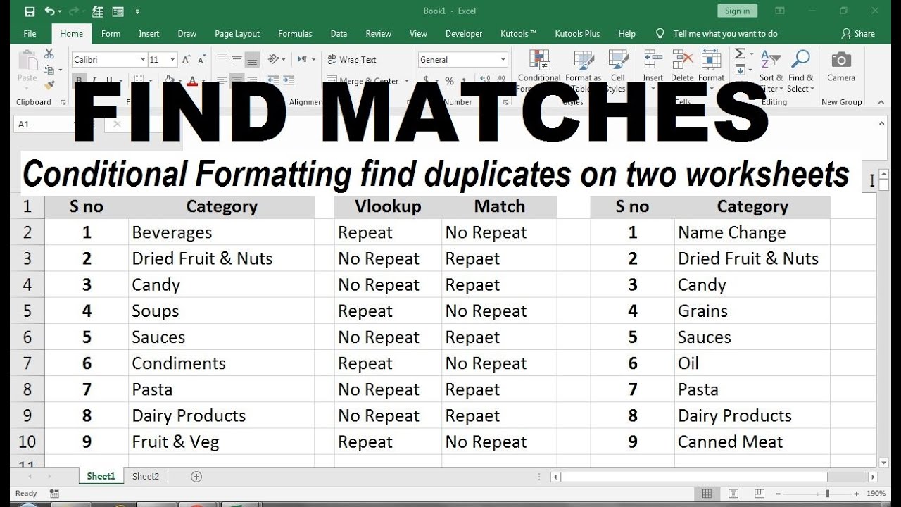
3. Conditional Formatting

Conditional Formatting can visually match data by highlighting cells that meet certain conditions:
- Navigate to the 'Home' tab, click on 'Conditional Formatting'.
- Choose 'New Rule' and then 'Use a formula to determine which cells to format'.
- Enter a formula to compare with the other sheet, like:
=A2=Sheet2!A2
- Set a format, like highlighting cells that match in green.
| Formatting Option | Description |
|---|---|
| Highlight Cells Rules | Use to highlight cells based on comparisons like equal to, greater than, etc. |
| Top/Bottom Rules | High or low values can be highlighted. |
| Data Bars | Visual representation of data by filling cells with bars. |
| Color Scales | Shade cells based on value relative to others. |

4. Power Query

For more advanced data matching, especially when dealing with large datasets or complex transformations, Power Query is invaluable:
- Go to 'Data' tab, click 'Get Data' or 'From Other Sources', then 'From Table/Range'.
- After loading the data from both sheets, use 'Merge Queries' to join on a common column.
- Apply transformations, like filtering, sorting, or grouping, to ensure your data matches precisely.
⚠️ Note: Ensure you understand the data structure before merging to prevent mismatched or incomplete data sets.
5. Using Microsoft Query or SQL

For users familiar with SQL or looking to leverage more powerful querying tools:
- From the 'Data' tab, select 'Get Data', then 'From Other Sources', and 'From Microsoft Query'.
- Connect to your Excel workbook and write SQL queries to join, filter, or manipulate data from both sheets.
- Example Query:
SELECT Sheet1.ID, Sheet2.Name
FROM `C:\Users\YourName\Desktop\Book1.xlsx` Sheet1
LEFT JOIN `C:\Users\YourName\Desktop\Book1.xlsx` Sheet2
ON Sheet1.ID = Sheet2.ID
As we conclude, matching data in Excel can be straightforward or complex depending on the tools you use and the nature of your data. The methods outlined above - from basic functions like VLOOKUP to advanced data manipulation with Power Query or SQL - provide a range of options for every level of user expertise. Choosing the right method depends on your comfort level with Excel, the volume of data, and the complexity of the required matching. By leveraging these techniques, you can ensure your datasets are aligned correctly, facilitating more accurate analysis and reporting.
What is the difference between VLOOKUP and INDEX/MATCH?

+
VLOOKUP can only look to the right of the lookup value in a table, whereas INDEX/MATCH can look both left and right, providing greater flexibility in data lookup and retrieval.
Can I use these matching techniques for sheets in different workbooks?

+
Yes, these techniques work across different workbooks by referring to the workbook, sheet, and range correctly, e.g., =[OtherWorkbook.xlsx]SheetName!A1
What should I do if VLOOKUP returns #N/A?

+
This error means no match was found. You might use IFERROR to handle this by specifying what to return or display instead of the error, like =IFERROR(VLOOKUP(…), “No Match”).
Is it better to use Power Query or manual formulas for large datasets?

+
For large datasets, Power Query is often more efficient as it performs calculations outside of the Excel grid, reducing performance issues and allowing for more complex transformations.


