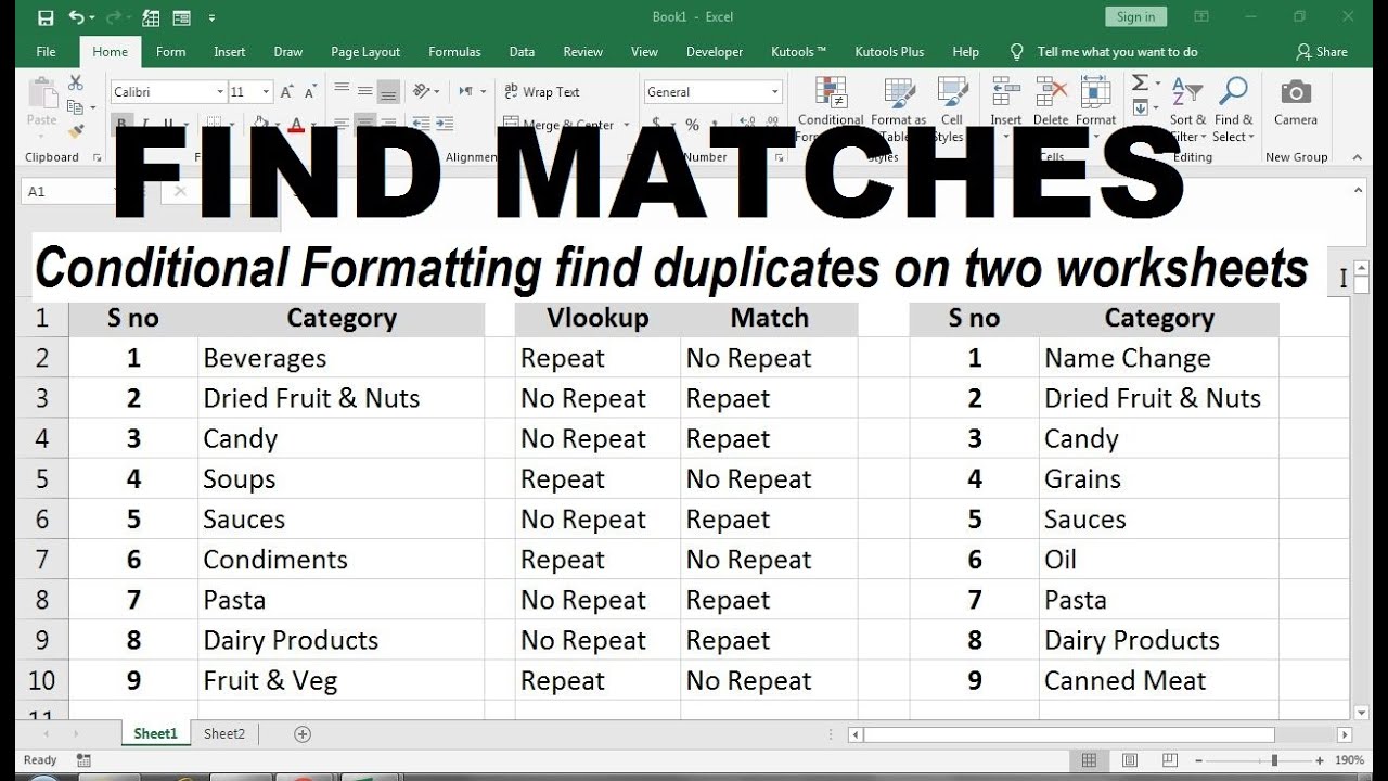
5 Proven Methods to Match Excel Sheets Seamlessly

Whether you're a data analyst, accountant, or just someone who works with numbers, Excel has long been the go-to tool for managing data. However, matching data across different sheets can often become a tedious task, prone to errors and oversights. Today, we will explore five proven methods to seamlessly match Excel sheets, enhancing your data management prowess and ensuring accuracy in your workflows. These techniques will not only save you time but will also maintain data integrity across your datasets.
Method 1: Using VLOOKUP for Simple Lookups

VLOOKUP is perhaps the most straightforward function for matching data in Excel. Here’s how you can use it:
- Identify the common key between your sheets, like an ID or a unique identifier.
- Enter the VLOOKUP formula in a new column in your destination sheet. The basic syntax is:
VLOOKUP(lookup_value, table_array, col_index_num, [range_lookup]) - Set range_lookup to FALSE for exact matches.
- Drag the formula down to fill the column or use the fill handle.
Method 2: INDEX and MATCH for More Flexibility

While VLOOKUP is useful, INDEX and MATCH provide greater flexibility, especially when dealing with column insertions or dynamic data:
- Use MATCH to find the position of your lookup value within a specified array.
- Then, employ INDEX to retrieve the value from that position in another array.
- The formula structure would be:
=INDEX(array, MATCH(lookup_value, lookup_array, [match_type]))
🚩 Note: INDEX-MATCH returns values without any reference, making it safer than VLOOKUP for error handling.
Method 3: Power Query for Advanced Matching

Power Query, available in Excel 2016 and later, offers a robust way to merge and clean data:
- Open the Power Query Editor from the Data tab.
- Load your data into Power Query.
- Use the Merge Queries option to join sheets on a common column.
- Expand the merged table to show desired columns.
- Apply transformations as needed before loading back into Excel.
Here’s an example of how your merged data might look in a table:
| ID | Name | Sheet1_Data | Sheet2_Data |
|---|---|---|---|
| 001 | John | Marketing | Sales |
| 002 | Emma | HR | Null |

Method 4: XLOOKUP for Upgraded Functionality

XLOOKUP is the new kid on the block, offering several advantages over VLOOKUP and HLOOKUP:
- It can look left or right and can handle both vertical and horizontal arrays.
- The basic syntax is:
=XLOOKUP(lookup_value, lookup_array, return_array, [if_not_found], [match_mode], [search_mode]) - Specify what should happen if no match is found with if_not_found.
- Use match_mode and search_mode for additional customization.
Method 5: Using Excel Tables for Dynamic Matching

Converting your data into Excel Tables (not to be confused with HTML tables) can make matching easier:
- Select your data range and convert to a Table from the Insert tab.
- Use structured references in your formulas for dynamic updates.
- Create relationships between tables using the Data Model feature.
- This approach supports vlookups, index-match, and other functions with table column references for better manageability.
When wrapping up your data matching tasks, take a moment to reflect on the impact these methods have on your workflow. Not only do they improve efficiency, but they also reduce the likelihood of errors. These tools are invaluable in ensuring that your data is accurate, comprehensive, and ready for any analysis or reporting needs. The beauty of Excel is in its ability to adapt to various data handling scenarios, and by mastering these matching methods, you're well on your way to becoming an Excel wizard.
What if my lookup value isn’t unique in the source sheet?

+
When dealing with non-unique lookup values, functions like VLOOKUP or XLOOKUP will return the first match they encounter. To handle multiple matches, consider using filter or Power Query for a more comprehensive solution.
Can I use these methods to match data from different workbooks?

+
Yes, these methods can work across different workbooks. For Power Query, you can load files into one query, and for formula-based methods, you can reference external workbooks in your formulas.
How do I deal with blank cells or errors in my source sheet?

+
You can use error handling functions like IFERROR or ISBLANK within your formulas to manage these scenarios. In Power Query, apply transformations to filter or replace null values as needed.


