5 Ways to Calculate Averages in Excel Sheets

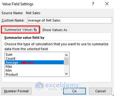
Calculating averages is a fundamental skill in data analysis, and Excel offers several methods to do so efficiently. Whether you're a student, a data analyst, or someone who loves numbers, understanding how to calculate averages in Excel can significantly streamline your workflow. This comprehensive guide will cover five different techniques to find averages, their applications, and tips for using them effectively.
1. The Basic AVERAGE Function

The simplest way to calculate an average in Excel is by using the AVERAGE function.
- Select the cell where you want to display the result.
- Type in =
AVERAGE(range), where range is the cell range you want to average.
💡 Note: The AVERAGE function ignores empty cells or cells with text, but will consider zeros.

2. AVERAGEIF: Condition-Based Averaging

If you need to calculate the average for a subset of data that meets certain conditions, AVERAGEIF is your go-to function.
- Syntax:
=AVERAGEIF(range, criteria, [average_range]) - range is where you’ll look for the criteria, criteria specifies what you’re looking for, and average_range is optional if different from the range you’re checking.
Example: Calculate the average of sales figures for a particular region:
=AVERAGEIF(B2:B100, “Region A”, C2:C100)3. AVERAGEIFS: Multiple Condition Averaging

For more complex averaging where multiple conditions need to be met, AVERAGEIFS allows you to average cells based on several criteria:
- Syntax:
=AVERAGEIFS(average_range, criteria_range1, criteria1, [criteria_range2, criteria2], …) - Here, average_range is the range where the average is computed, followed by criteria ranges and their respective criteria.
Example: Find the average sales for a particular region with sales above a threshold:
=AVERAGEIFS(C2:C100, B2:B100, “Region A”, C2:C100, “>1000”)
4. TRIMMEAN: Exclude Outliers

When dealing with datasets with potential outliers, the TRIMMEAN function helps you calculate an average by excluding a portion of data from both ends of the distribution:
- Syntax:
=TRIMMEAN(array, percent), where array is your data range and percent is the fraction of data to exclude from each end (expressed as a decimal).
Example: Trim the top and bottom 10% of sales data:
=TRIMMEAN(B2:B100, 0.1)
📊 Note: TRIMMEAN is particularly useful for financial analysis or any situation where outliers can significantly skew the average.
5. Manual Calculation Using SUM and COUNT

Sometimes, you might want to manually calculate the average using basic Excel functions:
- Sum up the values using
=SUM(range).
- Count the number of cells with numeric values using
=COUNT(range).
- Divide the sum by the count to get the average.
Example:
=SUM(A2:A100)/COUNT(A2:A100)
In conclusion, Excel provides numerous ways to calculate averages, each suited for different scenarios. From the straightforward AVERAGE function to the more advanced TRIMMEAN and AVERAGEIFS, understanding these methods allows you to tailor your data analysis to specific needs, ensuring you're making the most of your data with accuracy and efficiency.
What is the difference between AVERAGE and AVERAGEA in Excel?

+
The AVERAGE function calculates the arithmetic mean of numbers in a range, ignoring text or logical values. AVERAGEA, however, includes text and logical values in the average calculation, treating FALSE as 0, TRUE as 1, and text as 0.
How can I calculate the weighted average in Excel?

+
You can calculate the weighted average using the formula: =SUMPRODUCT(values, weights)/SUM(weights). Here, values are the numbers you want to average, and weights are their respective weights.
Why should I use TRIMMEAN instead of AVERAGE?

+
Use TRIMMEAN when your data might contain outliers or extreme values that could skew your average, giving you a more representative measure of central tendency by trimming the extremes.


