Easily Match Values in Excel Sheets with These Tips

Working with Excel can be a daunting task, especially when you have to juggle between multiple sheets or complex datasets. Often, one of the key activities in data analysis or management is to find and match values across different sheets. This not only helps in validating data but also in syncing up related information from various sources. Here are some easy tips to efficiently match values in Excel sheets.
Using VLOOKUP to Match Values


The VLOOKUP function is a go-to tool for matching data:
- Formula: =VLOOKUP(lookup_value, table_array, col_index_num, [range_lookup])
- Ensure the lookup_value (the value you want to find) is in the leftmost column of the table_array.
- Set the col_index_num to the column number from which you want the result.
🔍 Note: If the exact match does not exist, VLOOKUP can return an error or an approximate match depending on the last parameter, which you can set to FALSE for exact matches or TRUE/Omitted for approximate matches.
Combining INDEX and MATCH Functions


For more control and accuracy, consider combining INDEX and MATCH:
- INDEX Formula: =INDEX(array, row_num, [column_num])
- MATCH Formula: =MATCH(lookup_value, lookup_array, [match_type])
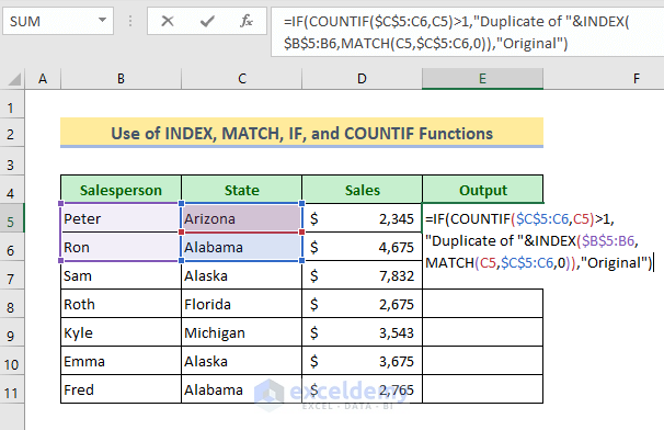
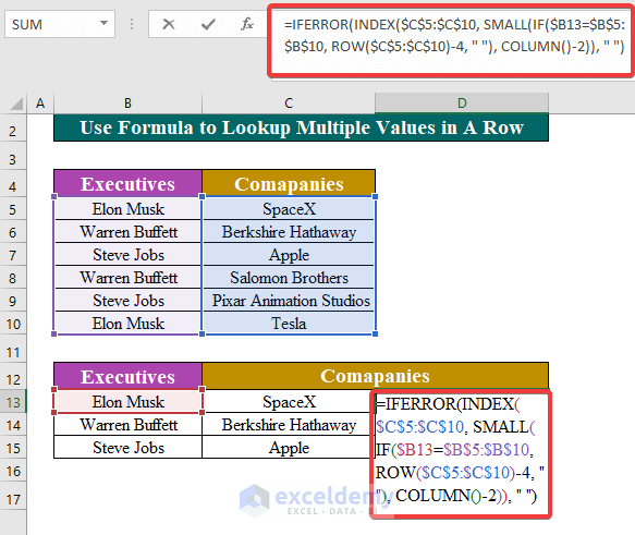
- Use MATCH to find the row number of the match, then feed that to INDEX to retrieve the data.
| Function | Description | When to Use |
|---|---|---|
| VLOOKUP | Look for a value in the leftmost column and return a value in the same row from a specified column. | Simple lookups where the lookup column is on the left. |
| INDEX & MATCH | More flexible lookup; finds the position and then retrieves data from that position. | Complex lookups, lookups from right to left, or when you need to change the lookup reference. |

Leveraging Power Query for Advanced Matching


Excel’s Power Query (Get & Transform) provides powerful tools for matching:
- Merge Queries: This allows you to join two tables based on common values.
- Transform Data: You can clean, transform, or filter data before matching.
💡 Note: Power Query is particularly useful when dealing with large datasets or when you need to perform recurring data matching tasks.
Using Conditional Formatting to Highlight Matches

Conditional formatting can visually indicate matches without needing formulas:
- Select the range where you want to highlight matches.
- Go to ‘Home’ > ‘Conditional Formatting’ > ‘New Rule’.
- Choose ‘Use a formula to determine which cells to format’ and enter a formula like =A2=B1 to highlight cells in column A that match a value in cell B1.
Using Lookup & Reference Tools


Excel offers several other tools for matching:
- XLOOKUP: Similar to VLOOKUP but with more flexibility.
- MATCH: Can be used standalone or combined with other functions.
- CHOOSE: To select from multiple ranges or arrays based on an index number.
By mastering these techniques, you not only streamline your data analysis workflow but also enhance the accuracy of your work. Whether you're performing quick lookups or managing large datasets, these tools can significantly boost your productivity in Excel.
What is the difference between VLOOKUP and XLOOKUP?

+
VLOOKUP looks for values in the leftmost column of a table and returns a value from the same row in a specified column, while XLOOKUP allows you to search from any column and has more default settings for error handling and lookups from both left to right or right to left.
Can I use Power Query for basic matching tasks?

+
Yes, Power Query can be used for basic matching tasks, especially when you need to match data across multiple files or when your matching criteria involve data transformations.
What if my data changes frequently? Do I need to recreate formulas?

+
If your data changes, you can use dynamic named ranges or table references in Excel, which will automatically adjust to data changes. Alternatively, using Power Query with refreshable connections ensures your matching operations are up-to-date with minimal effort.


