5 Simple Steps for VLOOKUP in One Excel Sheet

Mastering VLOOKUP in Excel can significantly enhance your ability to manage and analyze large datasets efficiently. This function allows you to search for a value in one column and return a corresponding value from another column. Here's a step-by-step guide to implement VLOOKUP on a single Excel sheet.
Step 1: Ensure Your Data is Structured Properly

Before you can use VLOOKUP, your data needs to be formatted in a table-like structure where each row represents a record, and columns contain specific data points. Here are the key points to ensure:
- Consistency: Make sure there are no blank rows or columns within the dataset you will be searching.
- Headings: Have clear headers for each column.
- Left to Right Flow: VLOOKUP will search from left to right, so the lookup value should be in the leftmost column of your data range.
Step 2: Identify Your Lookup Value and the Result Column

Identify which cell or column contains the value you want to look up and which column you want to pull data from:
- Lookup Value: This is the value you’re searching for within the first column of your data range.
- Result Column: The column where the value you want to retrieve is located.
Step 3: Write the VLOOKUP Formula

The VLOOKUP function in Excel uses the following syntax:
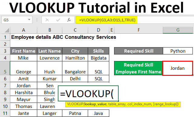
=VLOOKUP(lookup_value, table_array, col_index_num, [range_lookup])Here’s what each argument means:
| Argument | Description |
|---|---|
| lookup_value | The value you want to look up in the first column of the table array. |
| table_array | The range of cells that contains the data. |
| col_index_num | The column number within the table_array from which to retrieve the value. |
| [range_lookup] | A logical value: TRUE for an approximate match, FALSE for an exact match. |

To apply VLOOKUP:
- Start by typing
=VLOOKUPinto a cell where you want the result to appear. - Enter your lookup value in the first argument. For example, if the lookup value is in cell A2, you would type
=VLOOKUP(A2,. - Enter your data range. If your table starts at A1 and goes up to D100, you'd type
=VLOOKUP(A2, A1:D100,. - Specify the column index number. If you need data from the third column, use
3. Your formula now looks like this:=VLOOKUP(A2, A1:D100, 3. - Lastly, decide if you want an exact match (use
0orFALSE) or an approximate match (1orTRUE). For exact matches, your complete formula will be:=VLOOKUP(A2, A1:D100, 3, FALSE).
🚨 Note: Remember that VLOOKUP performs an approximate match by default, so setting the last argument to TRUE or omitting it might result in unexpected outcomes if the first column is not sorted.
Step 4: Adjust the Formula if Necessary

After entering the VLOOKUP formula:
- Check for Errors: If Excel returns #N/A or any other error, review your data, especially the lookup value and the table array range.
- Use Absolute References: If you plan to copy the formula across multiple cells, consider using absolute cell references (e.g., A1:D100) for the table_array to prevent Excel from changing the reference range when copied.
- Handle Case Sensitivity: VLOOKUP is not case sensitive, but if you need to match case, you can use helper columns with the EXACT function.
Step 5: Validate Your Results

Ensure the results of your VLOOKUP function are accurate:
- Spot Check: Manually verify a few results to ensure they match what you expect.
- Data Validation: Use data validation to limit lookup values to only those in your dataset to prevent #N/A errors.
- Test Against Known Values: Enter known values that should return specific results to check the formula’s accuracy.
🌟 Note: Using VLOOKUP with large datasets can slow down Excel, especially when performing an approximate match with unsorted data. Consider alternatives like INDEX and MATCH if performance is an issue.
The detailed steps provided above help you to utilize VLOOKUP effectively on a single Excel sheet. By following this process, you can streamline data analysis, ensure accuracy, and significantly enhance productivity. Whether you're matching inventory IDs, consolidating financial data, or reconciling client information, VLOOKUP is an indispensable tool for any Excel user.
Why does VLOOKUP return #N/A when I use it?

+
#N/A errors often occur because the lookup value doesn’t exist in the first column of your table array or because the table array reference is incorrect.
How can I make VLOOKUP more flexible?

+
Consider using the MATCH function combined with INDEX to achieve a more dynamic lookup function where columns can be added or removed without altering the formula.
Can VLOOKUP work with partial matches?

+
Yes, but not directly. Use wildcards like asterisk (*) or question mark (?) in your lookup value, or use helper columns with formulas like LEFT or RIGHT to match partial text.


