VLOOKUP Guide: Excel Sheets Data Match Made Easy

The VLOOKUP function in Excel is a powerful tool that allows you to search for a specific value within a table and return a corresponding value from another column. This function is particularly useful for looking up data in large datasets, matching and comparing information, or simply when you need to retrieve specific details quickly. Whether you're managing employee records, financial reports, or inventory lists, VLOOKUP can make your data management tasks easier and more efficient.
What is VLOOKUP?
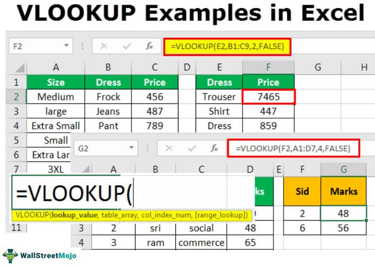
VLOOKUP stands for Vertical Lookup. It searches for a value in the first column of a range or table and returns a value in the same row from another column.
- It's ideal for looking up prices of items in a sales list, finding employee details in a large HR database, or matching customer information with their purchase history.
Here's the basic syntax for VLOOKUP:
VLOOKUP(lookup_value, table_array, col_index_num, [range_lookup])
- lookup_value: The value you want to find within your table.
- table_array: The range of cells that contains the data.
- col_index_num: The column number in the table from which to retrieve the value.
- range_lookup: TRUE for an approximate match or FALSE for an exact match (this parameter is optional).
How to Use VLOOKUP

Here’s a step-by-step guide to help you implement VLOOKUP in your spreadsheets:
Step 1: Set Up Your Data
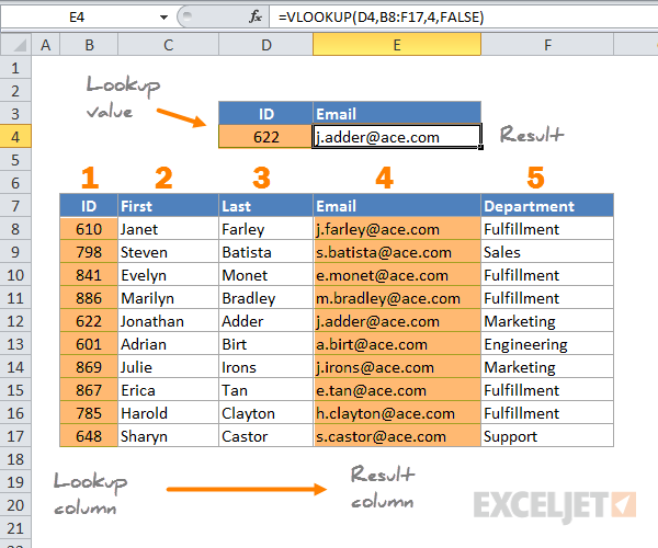

- Ensure your lookup column is the leftmost column in your table or range.
Step 2: Write the VLOOKUP Formula

- Select the cell where you want the result to appear.
- Enter the VLOOKUP formula:
In this example:=VLOOKUP(B2, A2:D10, 3, FALSE)- B2 is your lookup value.
- A2:D10 is your table array.
- 3 is the column number from which to return the value (in this case, the third column).
- FALSE indicates an exact match is required.
Step 3: Apply the Formula

- Once you've entered the formula, press Enter to see the result.
- If the formula returns an error, check for common issues like:
- Typographical errors in the lookup value.
- Incorrect column index number or table array selection.
- Ensuring the lookup value is present in the first column of the table array.
⚠️ Note: Always double-check your formula parameters; even a minor mistake can lead to unexpected results or errors.
Step 4: Handle Errors

VLOOKUP can return errors like #N/A if the lookup value is not found. Here are a few ways to handle these:
- Use the IFERROR function to return a custom message:
=IFERROR(VLOOKUP(B2, A2:D10, 3, FALSE), "Not Found") - For more advanced error handling, consider using the IF or ISNA functions in combination with VLOOKUP.
Advanced VLOOKUP Techniques

Dynamic Column Index
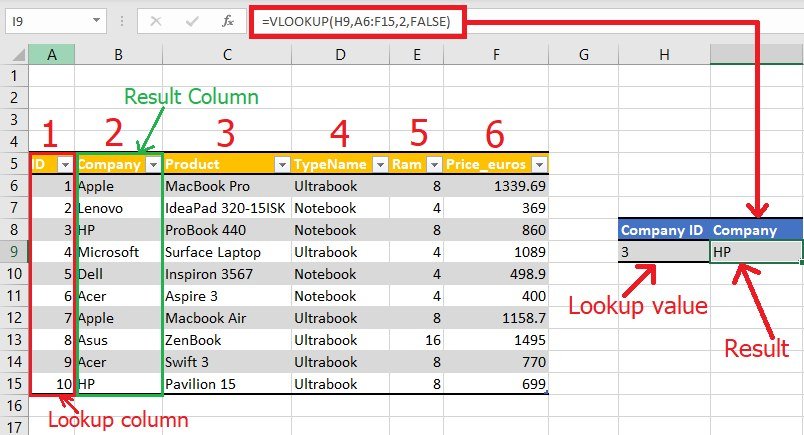
Instead of hardcoding the column index, you can use the MATCH function to dynamically find the column:
=VLOOKUP(B2, A2:D10, MATCH(“Item Price”, A1:D1, 0), FALSE)
- This allows your formula to automatically adjust if columns are inserted or deleted.
Approximate Match

Set the range_lookup argument to TRUE to allow for an approximate match. This is useful for graded data, like tax brackets or commission rates:
=VLOOKUP(A10, C2:D10, 2, TRUE)
Excel will look for the largest value less than or equal to the lookup value in the first column of your table.
📝 Note: When using an approximate match, ensure your table is sorted in ascending order by the first column.
Troubleshooting VLOOKUP Issues

Here are some common problems users face with VLOOKUP and how to resolve them:
- #N/A Error: The lookup value is not in the first column of your table, or it doesn’t match exactly.
- #REF! Error: Occurs when the col_index_num is greater than the number of columns in the table.
- #VALUE! Error: You might have specified a text lookup value in a formula expecting a number or vice versa.
| Error | Possible Cause | Solution |
|---|---|---|
| #N/A | Lookup value not found or formatting mismatch | Check the lookup value or use a wildcard (* or ?) if looking for a partial match |
| #REF! | Column index number exceeds table columns | Ensure the index number matches a column in the table |
| #VALUE! | Data type mismatch between formula and lookup value | Verify data types or use appropriate conversion functions |

Remember, regular maintenance and updates to your spreadsheets can prevent many of these common issues.
In the day-to-day data handling, the VLOOKUP function stands as an indispensable tool in Excel, streamlining data retrieval, analysis, and matching with ease. Its power to quickly locate and display relevant information from vast arrays of data simplifies complex tasks, reducing errors and saving time. By mastering this function, you’re equipped to manage large datasets effectively, ensuring accuracy and efficiency in your work. Whether you’re in finance, sales, or HR, VLOOKUP’s versatility makes it a must-know feature for any Excel user.
What is the difference between VLOOKUP with TRUE and FALSE range_lookup settings?

+
With FALSE, VLOOKUP searches for an exact match, which is more restrictive but ensures accuracy. TRUE allows for an approximate match, useful when dealing with continuous data like ranges or rates, but your data must be sorted in ascending order by the lookup column.
Can VLOOKUP return multiple values?
+
By itself, VLOOKUP returns a single result. However, you can use helper columns with formulas or functions like FILTER or INDEX/MATCH to return multiple values from multiple rows.
How do I handle errors in VLOOKUP?

+
Use the IFERROR function to wrap your VLOOKUP formula, which lets you define what Excel should display when VLOOKUP encounters an error, like a #N/A or custom text like “Not Found”.
Is VLOOKUP case-sensitive?

+
No, VLOOKUP is not case-sensitive. It matches values based on their content, not their case. If you need a case-sensitive lookup, consider using the EXACT function in a combination formula.
Can VLOOKUP search to the left?
+VLOOKUP cannot search to the left as it always looks for the lookup value in the first column of the table array. For left-sided searches, consider using INDEX and MATCH or the new XLOOKUP function in newer Excel versions.


