5 Ways to Find the Largest Number in Excel Quickly

Are you looking to streamline your data analysis in Excel by quickly identifying the largest number in a dataset? Whether you're handling financial reports, inventory management, or any data-centric task, knowing how to swiftly find the maximum value can save time and enhance productivity. Here are five effective methods to find the largest number in Excel with ease.
Method 1: Using the MAX Function

The MAX function is probably the simplest tool at your disposal for finding the largest number:
- Click on the cell where you want the result to appear.
- Type
=MAX(and select the range of cells you want to analyze. - Close the function with a parenthesis,
), and press Enter.
Excel will now display the largest value within the selected range. Here’s an example:

Method 2: Sorting and Filtering

If you need to see the context around the largest value or want to see all numbers in descending order:
- Select the range or column containing your data.
- Navigate to the Home tab, click on Sort & Filter, then choose Sort Largest to Smallest.
- The largest number will now be at the top of the column.
This approach is particularly useful when you want to rank or review data dynamically.
Method 3: Conditional Formatting

Conditional Formatting can visually highlight the largest number in a range:
- Select your data range.
- Go to Home > Conditional Formatting > Top/Bottom Rules > Top 10 Items...
- Set the dropdown to 1 and choose a format, then click OK.
This will format the largest number uniquely, making it stand out visually.
Method 4: Using the LARGE Function

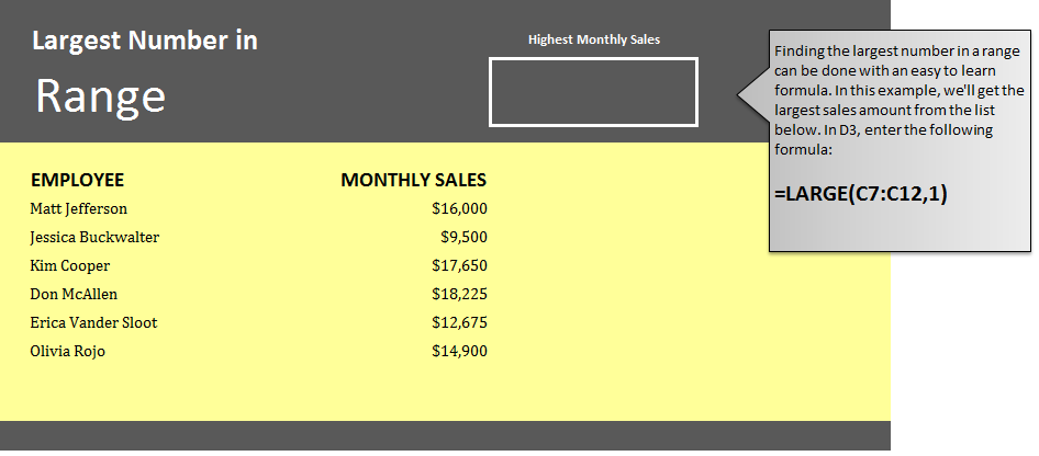
While not specifically for finding the largest number, the LARGE function can be adapted for this purpose:
- In the cell where you want the result, type
=LARGE(, select your range, then add a comma, 1). - Close the function and press Enter.
Here is an example:

💡 Note: The LARGE function can also be used to find the second, third, or any other nth largest value.
Method 5: Pivot Tables

For datasets with headers, pivot tables can be an incredibly powerful tool:
- Select your data range, go to Insert, and click on PivotTable.
- Choose where you want the PivotTable report to be placed.
- Drag the relevant field to the Row Labels area.
- Drag the same field to the Values area, right-click, and choose Value Field Settings.
- Select Max as the value aggregation function.
This approach not only finds the maximum value but also allows for further data analysis and reporting.
By utilizing these methods, you can efficiently locate the largest number in your Excel sheets, improving data analysis workflow and decision-making processes. Each method provides a different perspective, allowing you to choose the one that best fits your current needs or data presentation goals. These techniques empower you to work smarter with Excel, turning raw data into actionable insights with minimal effort.
How can I quickly identify the largest number in a large dataset in Excel?

+
Using the MAX function is the quickest way. Simply type =MAX(range) in the formula bar where range is your dataset. Press Enter, and Excel will return the largest value.
Can sorting be used to find the largest number?

+
Yes, sorting your data from largest to smallest will place the largest number at the top, but it changes the original order of your data.
Is there a way to highlight the largest number without changing the dataset?

+
Conditional Formatting can be used to highlight the top number in your dataset, visually identifying it without altering the data.
What if I want to find multiple largest values in a dataset?

+
Use the LARGE function, specifying the nth largest value you’re interested in by adjusting the second parameter; e.g., =LARGE(range,2) gives the second largest.


