5 Simple Ways to Compare Excel Sheets with Vlookup

In the dynamic world of data management and analysis, Microsoft Excel remains a cornerstone for many professionals across various industries. Its robust functionalities enable users to manipulate, analyze, and visualize data with ease. One of the most common tasks you might encounter when working with Excel is comparing data across different sheets. Whether it's reconciling financial reports, merging customer databases, or checking for discrepancies, knowing how to effectively compare Excel sheets can streamline your workflow significantly.
Understanding VLOOKUP for Data Comparison

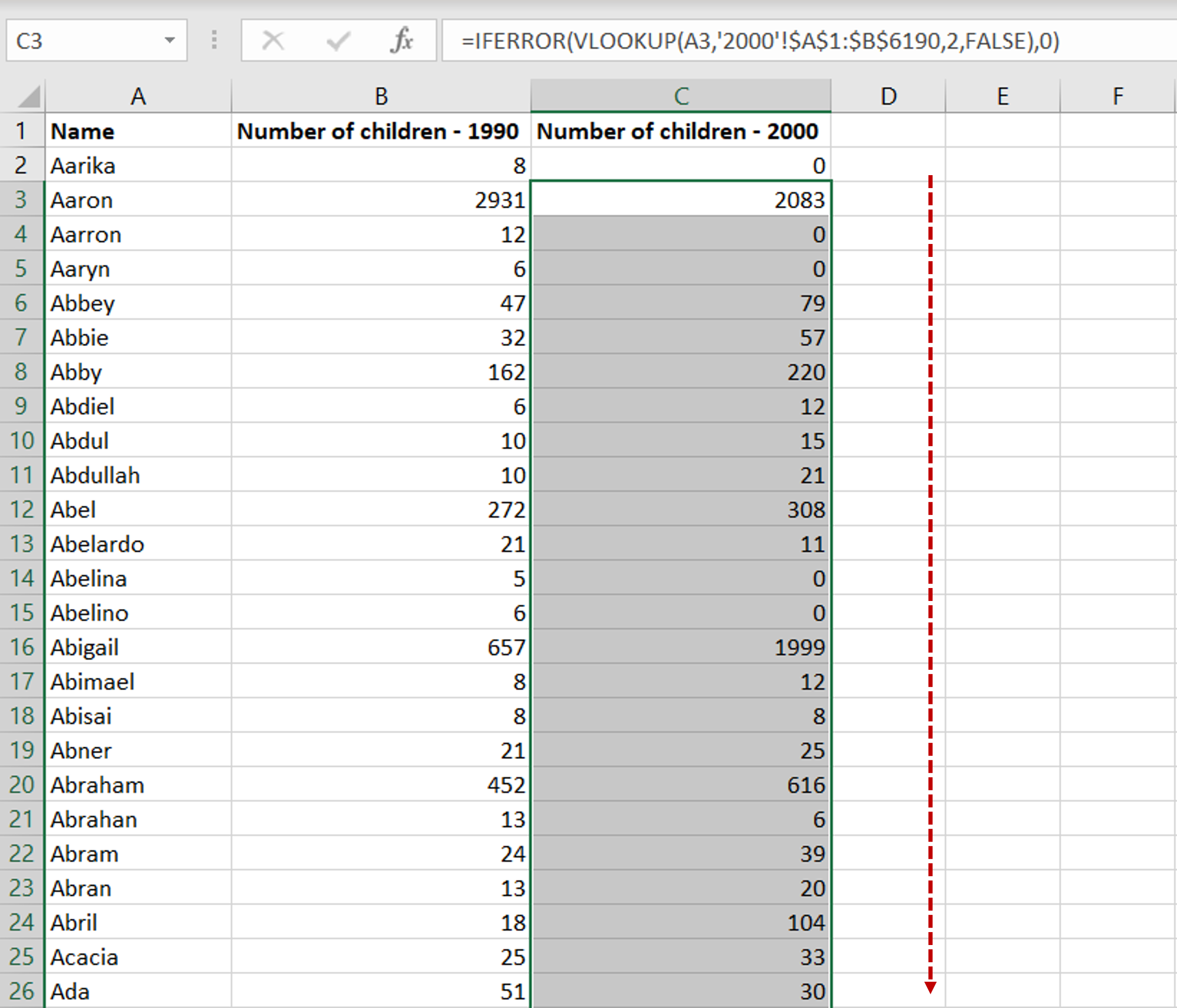
VLOOKUP (Vertical Lookup) is an Excel function that allows you to search for a value in the first column of a table array and return a value in the same row from another column. Here's how you can use VLOOKUP for comparing sheets:
Basic VLOOKUP Syntax

- =VLOOKUP(lookup_value, table_array, col_index_num, [range_lookup])
- lookup_value: The value you want to search for.
- table_array: The range of cells that contains the data.
- col_index_num: The column number in the table from which to retrieve the value.
- [range_lookup]: A TRUE/FALSE value indicating if you want an exact match or an approximate match.
⚠️ Note: By default, VLOOKUP assumes the lookup value is in the first column of the table array.
Steps to Compare Sheets Using VLOOKUP

1. Identify Common Keys

Before you start comparing, identify a common identifier or key that exists in both sheets. This could be an invoice number, employee ID, or any unique identifier.
2. Organize Your Data

- Ensure both sheets are structured similarly, especially in terms of the key you will use for comparison.
3. Apply VLOOKUP

Here’s how to apply VLOOKUP:
- Select a cell in Sheet 2 where you want to display the comparison result.
- Enter the VLOOKUP formula:
=VLOOKUP(A2,Sheet1!A2:B100,2,FALSE) - Here, A2 is your lookup value in Sheet 2.
- Sheet1!A2:B100 is the range on Sheet 1 where the lookup will occur.
- 2 indicates you want to return a value from the second column of this range.
- FALSE ensures you get an exact match.
4. Interpret the Results

- If the result of the VLOOKUP function matches the data in Sheet 2, then the values correspond to each other.
- If there’s an error, like #N/A, it means no match was found.
5. Validate Data Integrity

- Compare the total number of rows or unique identifiers across sheets.
- Look for anomalies or outliers by sorting or filtering the data post VLOOKUP application.
| Action | Description |
|---|---|
| Sort Data | Helps in quickly identifying missing or mismatched entries. |
| Filter Data | Allows you to focus on specific subsets of data for detailed comparison. |

Advanced Usage of VLOOKUP

Multiple Criteria Lookup

You can combine VLOOKUP with other functions like CONCATENATE to look up values based on multiple criteria:
- Example:
=VLOOKUP(CONCATENATE(A2,B2),Sheet1!A2:C100,3,FALSE)
Dynamic Range Lookup

Use named ranges or dynamic arrays to make your VLOOKUP formula adapt to changes in your dataset:
- Example:
=VLOOKUP(A2,Table1,2,FALSE)
🔍 Note: Excel's dynamic array functionality is available from Office 365 Excel version, enhancing the capabilities of traditional functions.
Conclusion

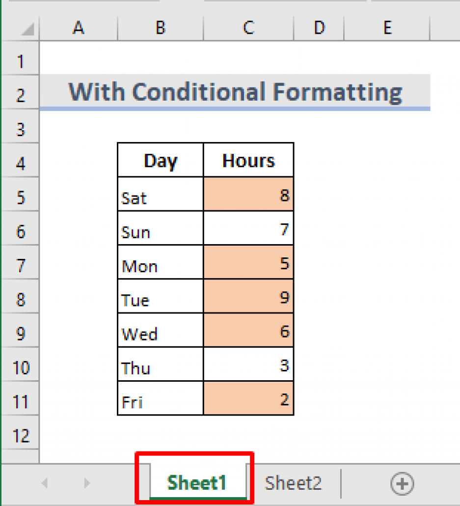
Mastering the use of VLOOKUP for comparing Excel sheets not only boosts your efficiency but also enhances your data analysis skills. By implementing these methods, you’ll be able to quickly identify discrepancies, perform accurate data reconciliation, and ensure data integrity across multiple spreadsheets. Remember, VLOOKUP is just one of many tools Excel offers for data comparison; exploring other functions like INDEX-MATCH or using conditional formatting can further augment your analytical prowess.
What if my lookup value isn’t in the first column of the table array?

+
In this case, you might need to use INDEX-MATCH instead, which doesn’t have this limitation.
How can I handle approximate matches with VLOOKUP?

+
By setting the range_lookup argument to TRUE, VLOOKUP will find an approximate match, useful for sorted ranges.
Can VLOOKUP return multiple values?
+VLOOKUP traditionally returns a single value. However, you can use helper columns or array formulas to achieve multiple value returns.


