3 Easy Ways to Combine Excel Data From Different Sheets

Combining data from different sheets in Excel can streamline your workflow, save time, and enhance data analysis. Whether you're dealing with financial data, sales reports, or any other type of information, Excel offers multiple methods to merge data from different sources. Here, we'll explore three easy and effective ways to combine Excel data from different sheets.
Method 1: Using Paste Link

The Paste Link feature in Excel allows you to create a dynamic link between cells in different sheets or workbooks. Here’s how you can use it:
- Select the cell or range of cells in the source sheet you want to link to the destination sheet.
- Copy the selected cells by pressing Ctrl + C.
- Navigate to the destination sheet where you want the data to appear.
- Right-click the top-left cell where you want to paste the data and select 'Paste Link' from the 'Paste Options' menu.
- Alternatively, you can also use Alt + E, S, then press F to paste a formula link.
This method creates a formula in the destination sheet that refers back to the original data. For example, if you paste link data from 'Sheet1!A1' into 'Sheet2!B1', you will see '=Sheet1!A1' in the formula bar when selecting 'Sheet2!B1'.
💡 Note: Any changes in the source cells will automatically update in the linked cells, ensuring data consistency across sheets.
Method 2: Using VLOOKUP and HLOOKUP Functions

If you need to combine data based on a common identifier, functions like VLOOKUP or HLOOKUP come in handy. Here’s a simple example:
- VLOOKUP: This function searches for a value in the first column of a range and returns a value in the same row from another column. Here’s how it works:
- Select the cell where you want the result to appear.
- Enter the VLOOKUP formula:
=VLOOKUP(lookup_value, table_array, col_index_num, [range_lookup]). - lookup_value is what you’re searching for.
- table_array is the range that contains the data.
- col_index_num is the column number from which to retrieve the value.
- range_lookup can be TRUE or FALSE to specify exact or approximate match.
- HLOOKUP: Similar to VLOOKUP, but searches for a value in the first row and returns a value from the same column. The syntax and parameters are similar except it uses row_index_num instead of col_index_num.
These functions are particularly useful when you want to pull data from another sheet based on matching criteria.
🔍 Note: VLOOKUP or HLOOKUP are not dynamic; if columns or rows are inserted or removed in the table array, you might need to update your formulas.
Method 3: Using Power Query

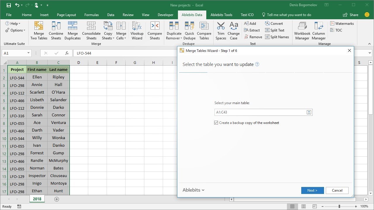
Power Query, available in Excel 2016 and later versions, is a powerful tool for data transformation and combining data from multiple sources:
- Open Excel and go to the 'Data' tab, then click on 'Get Data'.
- Select 'From File' then 'From Workbook' and choose your workbook.
- In the 'Navigator' window, select the sheets you wish to combine. You can use 'Ctrl' to select multiple sheets.
- Once selected, click 'Transform Data' or 'Load'. If you choose 'Transform Data', you'll enter the Power Query Editor.
- Here, you can append or merge queries:
- Append: Add data from one query to another. Go to 'Home' > 'Append Queries'. This is useful when combining sheets with similar structures.
- Merge: Combine data based on a common column. Go to 'Home' > 'Merge Queries', select the columns to merge on, and choose how you want to join the data.
| Operation | Use Case |
|---|---|
| Append Queries | When datasets have the same structure but different content. |
| Merge Queries | When datasets have related data that you want to combine based on matching fields. |

⚙️ Note: Power Query creates a connection to your data source, meaning changes in the source will be reflected in your Excel sheet, providing dynamic data refreshing capabilities.
In this comprehensive guide, we’ve covered three key methods to combine data from different sheets in Excel, each suited to different needs:
- Paste Link for quick and simple linking of data from one sheet to another, ensuring real-time updates.
- VLOOKUP/HLOOKUP for when you need to retrieve and combine data based on a common identifier or value.
- Power Query for powerful, flexible data manipulation and merging from multiple sources.
By employing these techniques, you can efficiently manage large datasets, enhance your data analysis, and maintain the integrity of your information across multiple sheets. Whether you’re merging customer information, aggregating financial data, or synthesizing sales figures, these methods provide a robust framework for working with Excel.
Remember, the choice of method depends on your specific requirements: - If you need to keep data synchronized across sheets, the Paste Link method or Power Query is optimal. - For data extraction based on specific criteria, VLOOKUP or HLOOKUP are your go-to tools. - When dealing with complex transformations or merging of multiple data sources, Power Query’s advanced capabilities make it indispensable.
These tools not only streamline your data management tasks but also open up possibilities for deeper data analysis and reporting. By mastering these methods, you’ll find Excel to be an even more powerful tool for your data handling needs.
What is the difference between VLOOKUP and HLOOKUP?

+
VLOOKUP searches for a value in the first column of a table and returns a value in the same row from another column. HLOOKUP, on the other hand, searches for a value in the first row and returns a value from the same column. Essentially, VLOOKUP is vertical, and HLOOKUP is horizontal.
Can Power Query handle multiple sheets?

+
Yes, Power Query can handle multiple sheets from the same or different Excel workbooks. You can load data from multiple sheets and then use append or merge functions to combine them as needed.
What happens if the source data linked via Paste Link changes?

+
Any changes made to the source data will automatically reflect in the destination cells where you used Paste Link, ensuring data consistency across different sheets or workbooks.


