Mastering Excel: How to Link Sheets with Formulas Easily

Linking sheets in Microsoft Excel using formulas not only enhances efficiency but also ensures data consistency across your spreadsheet workbook. Whether you're compiling data for financial reports, managing inventory, or organizing large sets of information, knowing how to link sheets properly is fundamental for effective data management.

Understanding the Basics of Sheet Linking

Before we dive into the practical steps, let’s understand why linking sheets is beneficial:

• Data Integrity: Ensures that changes in one cell or sheet automatically update all dependent cells.
• Time-Saving: Reduces the need for repetitive data entry and manual updates.
• Error Reduction: Minimizes the chance of human errors that occur during data replication.

Step-by-Step Guide to Linking Sheets

Here’s how you can link sheets in Excel:

1. Open Your Excel Workbook

   
   

   Start by opening the workbook containing the sheets you want to link.

2. Navigate to the Source Sheet

   
   

   Click on the tab of the sheet that contains the data you wish to link from, known as the “source” sheet.

3. Select and Copy the Source Cell

   
   

   Click on the cell or range of cells you want to link. Copy this selection by pressing Ctrl + C.

4. Navigate to the Destination Sheet

   
   

   Click on the tab of the sheet where you want the data to be linked, the “destination” sheet.

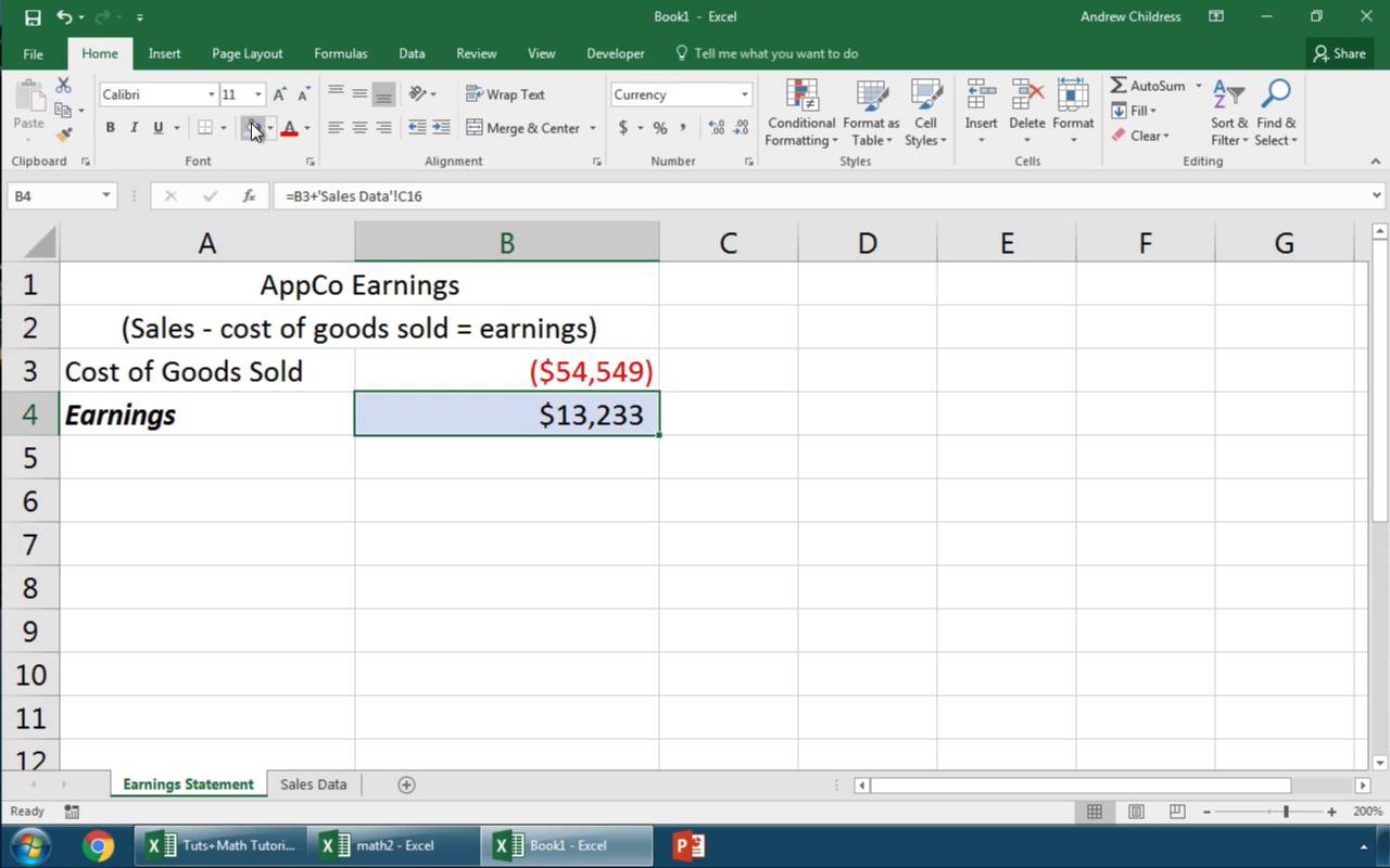
5. Use the Formula

   
   

   Instead of pasting directly, we’ll use a formula to create a link:

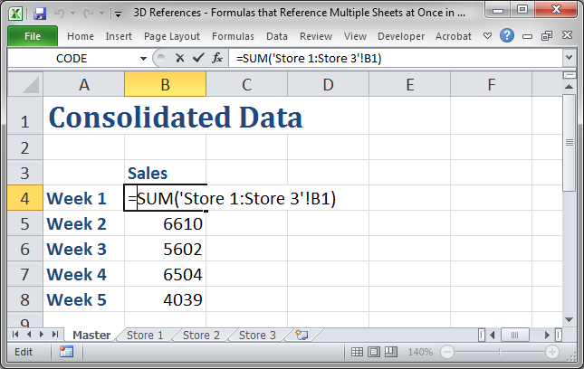
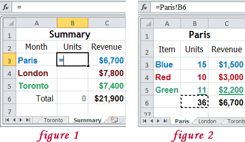
   =SheetName!CellReference

   For example, to link cell B3 from “Sheet1” to another cell in “Sheet2”, type:

   =Sheet1!B3

   Press Enter to complete the formula entry.

6. Verify the Link

   
   

   Check that the cell in the destination sheet now displays the content from the source sheet.

⚠️ Note: Ensure that the sheet names are exactly as they appear in your workbook, including spaces and case sensitivity. If you rename a sheet, you must update all formulas linking to it.

Advanced Techniques for Sheet Linking

Dynamic Sheet Naming

If you often change sheet names or need to link to dynamically named sheets, you can use:

=INDIRECT(A1 & “!” & B1)

• Cell A1 should contain the sheet name, and B1 the cell reference.
• This method avoids breaking links when sheet names change.

Linking Multiple Cells with Arrays

For bulk linking, use array formulas:

={Sheet1!A1:A10}

This will link a range of cells from A1 to A10 in “Sheet1” to the same range in the destination sheet.

💡 Note: Array formulas require Ctrl + Shift + Enter to be entered, not just Enter.

Troubleshooting Common Issues

Broken Links

Broken links occur when:

• The source sheet or cell reference does not exist or is renamed.
• The workbook is not saved in the same location.

Resolving involves checking the path or renaming references to match the updated information.

#REF! Errors

Encountering #REF! in your linked cells indicates:

• The source cells have been deleted.
• A sheet referenced in the formula has been deleted.

Rectify by restoring the original data or updating the formula to reflect current workbook structure.

🔧 Note: Regularly update or backup your workbook to prevent data loss due to linking errors.

In summary, linking sheets in Excel with formulas streamlines data management, ensuring accuracy and consistency across multiple worksheets. By mastering the techniques outlined above, you enhance your Excel proficiency, allowing for better data organization and analysis. Whether you’re handling financial models, tracking inventory, or managing any form of complex data, these skills are invaluable.