5 Easy Steps to Add a Pivot Table in Excel

Ever found yourself drowning in heaps of data, struggling to make sense of the numbers? Microsoft Excel's pivot table feature might just be the lifeboat you need. In this post, we'll go through 5 straightforward steps to add a pivot table to your Excel sheet, enabling you to summarize, analyze, and explore your data with ease. Let's dive in!
Step 1: Prepare Your Data

Before you start creating your pivot table, your data must be organized correctly:
- No Blank Rows or Columns: Ensure there are no completely empty rows or columns within your data set.
- Headers: Each column should have a unique header to serve as the field names for your pivot table.
- Uniform Data: The data in each column should be consistent in type; numbers should be numbers, dates should be dates, and so on.
🚫 Note: If your data is not formatted correctly, the pivot table might not function as expected, so take the time to clean up your data first.
Step 2: Select Your Data

Here’s how to select your data range for the pivot table:
- Click on any cell within your data set.
- Press Ctrl + A to select all data, or manually drag to select the desired range.
- Keep in mind that you can always adjust the data range later if needed.
Step 3: Insert the Pivot Table

Now, let’s create the pivot table:
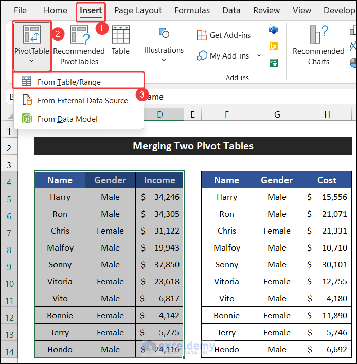
- Go to the Insert tab in Excel’s ribbon.
- Click on PivotTable to open the Create PivotTable dialog box.
- Select if you want the pivot table to be placed in a new worksheet or an existing one.
Step 4: Set Up Your Pivot Table

With your pivot table inserted, it’s time to configure it:
- Drag the fields from the field list to one of the four areas: Rows, Columns, Values, or Filters.
- Rows: Fields to categorize data vertically.
- Columns: Fields for horizontal categorization.
- Values: Fields to summarize or perform calculations on.
- Filters: Fields that control which data is shown or hidden.
⚙️ Note: Experiment with different arrangements to find the most insightful view of your data.
Step 5: Analyze and Refine

With your pivot table set up, you can now:
- Sort, filter, or drill down into the data to gain deeper insights.
- Create visual representations like pivot charts to make the data more digestible.
- Use additional features like Slicers or Timeline to interact with the data more dynamically.
Excel provides an intuitive Analysis tab specifically for pivot tables, giving you easy access to these features:
| Feature | Description |
|---|---|
| Expand/Collapse | Show or hide detailed data to keep your report focused. |
| Field Settings | Change how data is summarized or formatted within your pivot table. |
| Slicer | Use slicers for filtering data with a graphical interface. |

🔍 Note: Regularly update your pivot table data by refreshing it when the source data changes.
By following these steps, you've turned a sea of numbers into a clear, concise, and interactive summary. Whether for business analytics, financial reporting, or simply organizing personal data, pivot tables in Excel provide a powerful tool for data analysis. This process not only streamlines your workflow but also opens up new avenues of insight that can inform decisions and drive strategy.
Can I use pivot tables for non-numeric data?

+
Absolutely! Pivot tables can count, show unique values, and provide various calculations for text data, not just numbers.
How do I refresh my pivot table?

+
Right-click on any cell in your pivot table and select Refresh, or use the keyboard shortcut Alt + F5.
What if my data changes?

+
Refresh the pivot table to reflect any changes in the source data. You might also need to change the data source if you’ve added new columns or rows.
Can I customize the design of my pivot table?

+
Yes, you can customize the layout, design, and formatting options through the PivotTable Tools > Design tab.
What are some common pitfalls to avoid when creating pivot tables?

+
Ensure your data is clean and well-organized, avoid using formulas in your data that change when filtered, and be cautious about expanding your data without updating your pivot table range.


