5 Ways to Highlight Data in Excel Sheets

Excel, a powerful tool within Microsoft Office Suite, is renowned for its data manipulation capabilities. Whether you're analyzing sales figures, tracking inventory, or organizing event schedules, knowing how to effectively highlight key data can significantly enhance your productivity and presentation. Here are five effective methods to highlight data in Excel sheets, making your data stand out for better analysis and decision-making.
1. Conditional Formatting

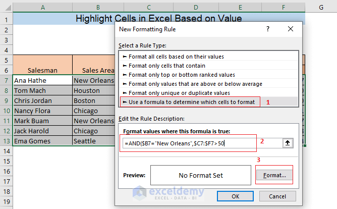
Conditional Formatting allows you to automatically format cells with a color, font style, or icons based on the cell’s value. This feature is incredibly versatile:
- Data Bars: Represent the value of a cell relative to other cells in the range, visually extending into the cell with bars.
- Color Scales: Assign different colors to cells based on their values, creating a gradient effect that can show trends at a glance.
- Icon Sets: Use icons to categorize data (e.g., flags, arrows, or shapes) to quickly indicate status or priority.

To apply conditional formatting:
- Select the cells you wish to format.
- Go to the 'Home' tab, then click 'Conditional Formatting' in the 'Styles' group.
- Choose the type of rule you want to apply (e.g., 'New Rule' for custom settings).
- Set the rule, specify the formatting, and click 'OK'.
🖌 Note: Conditional Formatting automatically updates as data changes, making it dynamic for real-time analysis.
2. Using Cell Styles

Excel provides Cell Styles that are predefined formatting options which include font, alignment, and color settings. You can apply these to highlight data:
- Select the range or cells you want to style.
- Navigate to the ‘Home’ tab, then under ‘Styles’, click ‘Cell Styles’.
- Choose from the styles list like ‘Good’, ‘Bad’, ‘Neutral’, or create custom styles.
3. Highlight Cells Rules

Excel’s ‘Highlight Cells Rules’ are quick methods for spotlighting cells:
- Greater Than: Highlights cells with values above a certain number.
- Top/Bottom Rules: Show the top or bottom values, percentages, or above/below average.
- Equal To: Highlights cells with exact matches.
- Text that Contains: Use for text searches to highlight specific words or phrases.
This feature is extremely useful for quick visual analysis:
- Select your data range.
- From the ‘Home’ tab, go to ‘Conditional Formatting’ then ‘Highlight Cells Rules’.
- Choose your rule, set the criteria, and decide on the highlighting style (e.g., color, text color, etc.).
4. Data Validation with Custom Alerts

Besides highlighting, Data Validation can alert users if data does not meet specific criteria:
- Select the cells where you want to apply validation.
- Go to the ‘Data’ tab, choose ‘Data Validation’.
- Set up rules (e.g., whole numbers, list, date, etc.).
- In the ‘Input Message’ and ‘Error Alert’ tabs, you can define custom messages or alerts to highlight issues.
This method not only highlights but also enforces data entry standards.
5. Using Tables for Visual Distinction

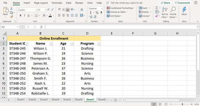
Tables offer an immediate way to highlight data with built-in styles and automatic banded rows:
- Auto-Filtering: Tables come with built-in filters, making data analysis interactive.
- Structured References: References to table data are more readable and maintainable.
To convert a range into a table:
- Select your data range.
- Go to the ‘Insert’ tab, click ‘Table’, or use Ctrl+T.
- Ensure ‘My table has headers’ is checked if your data includes headers.
In summary, the art of highlighting data in Excel revolves around several techniques that, when used wisely, can transform raw data into visually compelling insights. From Conditional Formatting for dynamic data representation to Tables for organized datasets, each method offers unique benefits for data visualization. These methods not only make your data easier to analyze but also facilitate better communication of your findings. Whether you're presenting to stakeholders or simply making sense of large data sets for internal use, mastering these techniques is crucial for leveraging Excel's full potential.
What is the benefit of using Conditional Formatting?

+
Conditional Formatting makes it easy to visually analyze data by highlighting or formatting cells based on certain criteria, providing instant visual cues that aid in quick decision-making and trend analysis.
Can I create custom styles for cells?

+
Yes, Excel allows you to create custom styles by selecting cells, going to the ‘Home’ tab, and choosing ‘New Cell Style’ under ‘Cell Styles’ to define your own formatting options.
How can Data Validation help highlight data?

+
Data Validation helps by preventing incorrect data entry through rules and alerts, thus indirectly highlighting data by ensuring accuracy and integrity in your dataset.
Is it possible to highlight an entire row based on a cell’s value?

+
Yes, with Conditional Formatting, you can set a rule to highlight an entire row based on the value in a specific cell within that row, using a formula to define the condition.
What happens when I change data in a table?

+
When you change data in an Excel table, the formatting and functionality of the table automatically adjust. The table will adapt to new rows, maintain banding, and update references to maintain data integrity and presentation consistency.


