5 Simple Steps to Create an Excel Chart

In today's data-driven world, visualizing information effectively is crucial for making informed decisions. Whether you're tracking sales, analyzing survey data, or managing inventory, Excel charts serve as a powerful tool to convey complex data through graphical representations. Here, we'll guide you through five simple steps to create an Excel chart, allowing you to present your data in a way that's both appealing and informative.
Step 1: Prepare Your Data

Before you dive into charting, ensure your data is well-organized:
- Data Entry: Enter your data into Excel. Each row should represent a record, and columns should denote variables.
- Sort and Clean: Arrange your data logically, remove duplicates or outliers, and fill in missing values where necessary.
- Naming: Clearly label each column to make chart creation smoother.
Step 2: Select Your Data

Choose the data you want to visualize:
- Highlight the relevant rows and columns. If you’re creating a chart for multiple data series, ensure your selection captures all necessary data points.
Step 3: Insert a Chart

With your data selected:
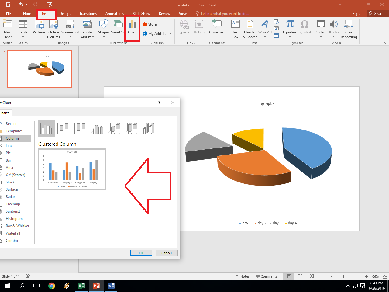
- Go to the “Insert” tab on the Excel ribbon.
- Click on the “Chart” group to reveal various chart options.
- Select the chart type that best represents your data, like a column chart for comparing values, a line chart for trends, or a pie chart for distribution.
Step 4: Customize Your Chart

Here’s where you can make your chart unique:
- Chart Elements: Add or remove chart elements like titles, axis labels, legends, and data labels.
- Style and Color: Choose a style, color palette, and font that aligns with your brand or presentation theme.
- Axis Adjustments: Modify axis scales, intervals, or even swap axes for better clarity.
Step 5: Analyze and Present Your Data

Once your chart looks the part:
- Data Interpretation: Interpret your chart to draw meaningful insights.
- Presentation: If you’re sharing your findings, consider using Excel’s features like data tables, trendlines, or annotations to enhance your presentation.
📌 Note: If your chart includes time-based data, Excel can format the axis as a timeline for clarity.
By following these steps, you can transform raw data into an insightful chart in Excel. Whether it’s for business analysis, academic research, or personal projects, this skill empowers you to tell stories through numbers, making your data more impactful and easier to understand.
Now, let’s summarize what we’ve covered:
Creating an Excel chart is more than just clicking through software; it's about strategically presenting your data to make it accessible and actionable. From selecting and preparing your data to customizing your chart for maximum impact, each step plays a vital role in the success of your visualization. Keep experimenting with chart types and styles to find the most effective way to convey your data's story. Here are some key takeaways:
- Good data preparation is essential before you chart.
- The choice of chart type is critical for accurate data representation.
- Customization can make your chart stand out and communicate more effectively.
- Analysis and interpretation of the chart help in drawing actionable insights.
What is the best chart type for comparing data over time?

+
A line chart is generally the best choice for visualizing data trends over time, as it clearly shows changes and continuity in data.
Can I create charts from multiple data series?

+
Yes, Excel supports charts with multiple data series. You can select multiple columns or rows when choosing your data to create a chart that includes several series.
What should I do if my chart looks cluttered?

+
Simplify your chart by reducing the number of series, choosing less cluttered chart styles, or using filters to focus on key data.


