5 Ways to Link Excel Cells Between Sheets

Connecting data across different sheets in Excel can transform the way you manage and analyze information. Whether you're tracking project milestones, syncing sales figures, or managing a household budget, knowing how to link Excel cells effectively can save time and increase accuracy. Here are five key methods to link Excel cells between sheets:
1. Direct Reference Linking

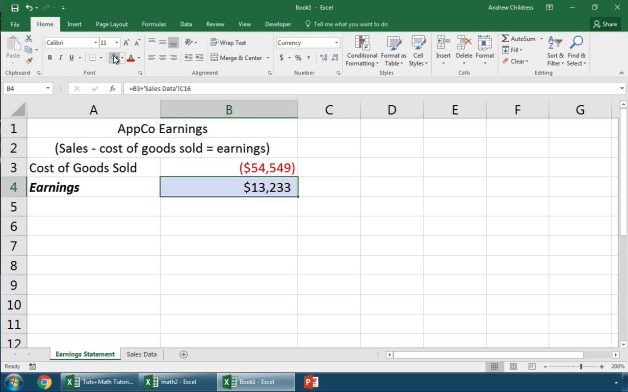
Direct Reference Linking is the simplest way to connect data across different worksheets. Here’s how you do it:
- Open both the source and the destination sheets in Excel.
- In the cell where you want to display the linked data, type an equal sign (=).
- Navigate to the source sheet by clicking its tab or using keyboard shortcuts like Ctrl + Page Up/Page Down.
- Select the cell you want to link, and press Enter. The formula bar will display something like
=Sheet2!A1.
🔍 Note: This method is best for static linking where the source data doesn’t move around the sheet.
2. Named Ranges for Easy Navigation

Named Ranges can make navigating and linking data easier, especially in larger workbooks:
- Go to the cell you want to name.
- Select Formulas > Define Name from the ribbon.
- Name your cell or range.
- Then, on your destination sheet, type = and the name of the range. For example, if you named a cell ‘Total’, you would write
=Total.
Named Ranges not only make formulas more readable but also adapt if the source data’s position changes.
3. Using VLOOKUP Across Sheets

VLOOKUP is particularly useful for looking up data in different sheets based on a key value:
- In your destination sheet, start with the formula =VLOOKUP(
- Select the lookup value, then navigate to the source sheet and select the table array.
- Specify the column index number and choose FALSE for an exact match.
- The formula will look something like:
=VLOOKUP(A2,Sheet2!A1:D100,2,FALSE).
🌐 Note: VLOOKUP is great for databases where you need to pull related information from different sheets.
4. Data Consolidation

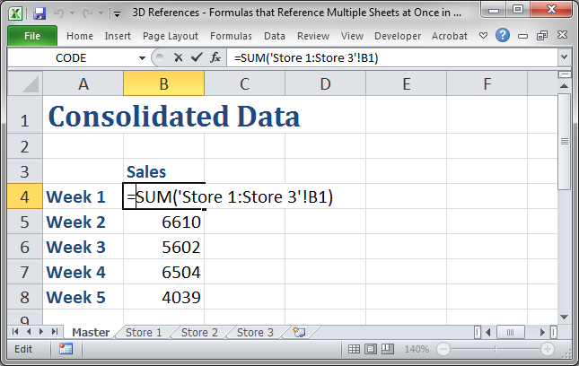
When you want to summarize data from multiple sheets or ranges, Excel’s Data Consolidation feature can be quite handy:
- Go to Data > Consolidate.
- Choose the function you need (Sum, Average, etc.).
- Add each range from different sheets by clicking in the “Reference” box and selecting the range.
- Press OK, and the consolidated data will appear in the destination sheet.
Here’s how this looks:
| Sheet Name | Cell | Data |
|---|---|---|
| Sheet1 | A1 | 10 |
| Sheet2 | A1 | 20 |
| Sheet3 | A1 | 30 |

⚙️ Note: Consolidation can simplify reporting from multiple data sources.
5. External Reference Links

For those working with multiple Excel files, linking between them is vital:
- Open both the source workbook and the workbook where you want to link the data.
- In the destination cell, type = followed by the path to the source file, sheet name, and cell.
- For example:
=‘C:\Users[USERNAME]\Documents[FILE_NAME.xlsx]Sheet1’!A1 - When linking, Excel will open the other workbook to validate the link.
In conclusion, mastering these methods of linking Excel cells between sheets can greatly enhance your efficiency in managing complex datasets. From simple static links to dynamic lookups, each method serves unique purposes. Understanding when and how to apply these techniques can transform your workflow, making it more streamlined and error-free. Now, with the ability to link and consolidate data at your fingertips, you can organize and analyze information in new, more insightful ways.
Can I link cells between sheets in different workbooks?

+
Yes, you can link cells between sheets in different workbooks using external references. Excel will update the links automatically when opening both workbooks.
What happens if the source data is moved or deleted?

+
If the source data changes location or is deleted, the linked cell will display an error. You’ll need to update the formula or remove the link.
How do I prevent accidental overwriting of links?

+
Lock cells with links by selecting them, right-clicking, choosing “Format Cells,” then under the “Protection” tab, uncheck “Locked.” Then, protect the sheet with “Review > Protect Sheet.”


