Master Excel VLOOKUP to Merge Two Sheets Easily

In today's data-driven world, mastering tools like Microsoft Excel can significantly enhance productivity and decision-making. One of the most powerful functions in Excel is VLOOKUP, which stands for Vertical Lookup. This function is indispensable for those who frequently deal with large datasets, especially when merging data from multiple sheets. This guide will take you through a step-by-step process to use VLOOKUP to merge two sheets seamlessly, making your data management tasks more efficient.
Understanding VLOOKUP

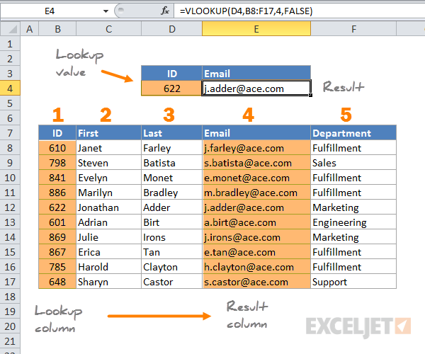
VLOOKUP is designed to search for a value in the first column of a range of cells and return a value in the same row from another column. Here’s a basic breakdown:
- It searches vertically down the first column of the table.
- It retrieves the value from the specified column in the same row.
Before You Begin

Ensure your data is:
- Well-organized with consistent formatting.
- Free from any merged cells that might interfere with lookup.
- Accurately labeled with headers for easy reference.
Step 1: Prepare Your Sheets

Before you start merging, prepare both sheets:
- Sheet 1 - This should be your primary data source. Ensure the column where you want to perform the VLOOKUP contains unique identifiers.
- Sheet 2 - This sheet should contain supplementary data you want to merge into Sheet 1. Make sure there’s a common identifier in one of the columns.
📌 Note: Both sheets must have a common identifier or key for VLOOKUP to work correctly.
Step 2: Write the VLOOKUP Formula

The VLOOKUP formula follows this syntax:
VLOOKUP(lookup_value, table_array, col_index_num, [range_lookup])
- lookup_value: The value you are looking for.
- table_array: The range of cells that contains the data.
- col_index_num: The column number in the table from which to retrieve the value.
- [range_lookup]: TRUE for an approximate match, FALSE for an exact match. Usually, we use FALSE.
Example:

| Customer ID | Name | Amount |
|---|---|---|
| 1001 | John Doe | 250 |
| 1002 | Jane Smith | 150 |

In Sheet 1, if you want to find the name corresponding to ID 1001 from Sheet 2, your formula would look like:
=VLOOKUP(A2,Sheet2!A1:C2,2,FALSE)
Here, A2 is the lookup value from Sheet 1, Sheet2!A1:C2 is the range on Sheet 2, 2 is the column index number for the name, and FALSE means you want an exact match.
Step 3: Apply VLOOKUP Across Columns

Now, let’s extend the VLOOKUP across all the relevant rows:
- In Sheet 1, in the cell where you want to pull data from Sheet 2, enter your VLOOKUP formula.
- Drag the formula down to apply it to all rows, or double-click the fill handle to auto-fill.
As you drag or copy the formula:
- Ensure that your lookup_value references the correct cell from Sheet 1.
- The table_array and col_index_num should remain constant or be adapted if merging multiple sheets.
Step 4: Handling Errors and Edge Cases

Here are some common issues you might encounter and how to address them:
- #N/A Error: This indicates that the VLOOKUP couldn’t find a match. Consider using
IFERRORto handle this gracefully, for example:
=IFERROR(VLOOKUP(A2,Sheet2!A1:C2,2,FALSE),“Not Found”)
📌 Note: VLOOKUP can be slow with large datasets. For big sheets, consider using INDEX-MATCH or the newer XLOOKUP function for better performance.
Advanced Techniques

Here are some tips for when you need more from your VLOOKUP:
- Dynamic Range: Use a named range or the OFFSET function for dynamic data.
- Double VLOOKUP: Combine two VLOOKUPs for a two-way lookup.
- Conditional Formatting: Use conditional formatting to highlight cells with errors or matches.
Merging sheets using VLOOKUP in Excel is a skill that, once mastered, can transform your data management workflow. From ensuring data consistency to simplifying complex tasks, VLOOKUP offers both beginners and advanced users powerful tools to manipulate and analyze data efficiently. Remember to keep your data clean, utilize error handling, and consider advanced techniques for larger datasets to get the most out of this function. Practice and experimentation will make you an Excel VLOOKUP pro, enabling you to merge data with confidence and ease.
What is the difference between VLOOKUP and XLOOKUP?

+
VLOOKUP searches vertically in the first column, whereas XLOOKUP can search both vertically and horizontally with more flexibility in terms of return values and error handling.
Can VLOOKUP work with unsorted data?

+
Yes, VLOOKUP can work with unsorted data as long as the exact match argument (FALSE) is used. However, sorting can improve lookup performance.
How can I speed up my VLOOKUP for large datasets?

+
Use Excel features like disabling automatic calculations, limiting the number of rows in your lookup range, or switch to functions like INDEX-MATCH or XLOOKUP for improved performance.


