5 Ways to Hyperlink Between Excel Sheets Easily

Excel, a tool widely used in both professional and personal settings, often involves managing and analyzing large sets of data across multiple sheets. Knowing how to hyperlink between these sheets can significantly streamline your navigation and enhance productivity. Here are five straightforward methods to create hyperlinks in Excel:
1. Using the HYPERLINK Function

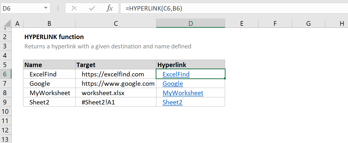
The HYPERLINK function in Excel allows you to link to another part of the document or to external files or web pages. Here’s how:
- Click the cell where you want to insert the hyperlink.
- Type the following function:
=HYPERLINK(“[SheetName]!CellAddress”, “Link Text”) - For example, to link to cell A1 in Sheet2, you’d write:
=HYPERLINK(“Sheet2!A1”, “Go to Sheet2”) - Press Enter. The cell now displays the link text, and clicking it will take you to the specified location.
💡 Note: Sheet names with spaces or special characters must be enclosed in single quotes, like this: =HYPERLINK("'[Sheet Name]'!A1", "Link Text")
2. Insert Hyperlink via Context Menu

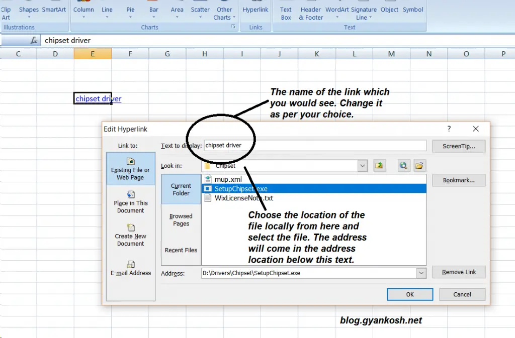
Instead of manually typing out the HYPERLINK function, you can use Excel’s context menu:
- Right-click on the cell where you want to add the hyperlink.
- Select Hyperlink or Link from the dropdown menu.
- Choose Place in This Document.
- Select the sheet and cell reference you want to link to.
- Enter link text, then click OK.
3. Creating Named Ranges

Named ranges provide a quick way to refer to specific data blocks:
- Select the cell range you wish to name.
- Enter the desired name in the Name Box (next to the formula bar).
- Use
=HYPERLINK(“[SheetName]!NamedRange”, “Link Text”)to link to this named range.
4. Using the Insert Function

This method involves using Excel’s function wizard:
- Click on the cell where you want the hyperlink.
- Go to the Formulas tab, click Insert Function.
- From the list, select HYPERLINK.
- Fill in the Link_Location as
[SheetName]!CellAddressand choose your link text.
5. Table of Contents with Hyperlinks

If you’re dealing with a workbook with many sheets, creating a table of contents can be useful:
- In a new sheet, list all the sheets you want to link.
- In an adjacent column, use the HYPERLINK function or insert a hyperlink for each sheet name, directing to cell A1 of that sheet.
| Sheet Name | Link |
|---|---|
| Sheet1 | =HYPERLINK(“Sheet1!A1”, “Sheet1”) |
| Sheet2 | =HYPERLINK(“Sheet2!A1”, “Sheet2”) |

💡 Note: Ensure that the sheet names match exactly or use Excel's name manager to create unique identifiers if you're working with similar sheet names.
Navigating through multiple Excel sheets can be made efficient and user-friendly with hyperlinks. These methods not only help in organizing data but also in quickly accessing relevant information, thereby saving time and reducing errors during data analysis. Remember, while hyperlinks are convenient, maintaining a consistent naming structure for your sheets and cells will make this process even smoother.
Can I hyperlink to a specific cell in another Excel sheet?

+
Yes, you can link to a specific cell using the HYPERLINK function or the Insert Hyperlink dialog. Simply include the exact cell address in your hyperlink formula or select it from the dialog box.
What if the linked sheet is deleted or renamed?

+
If the sheet is deleted or renamed, the hyperlink will break. Always double-check and update your links when making changes to your workbook structure.
How do I format the text of my hyperlink?

+
After inserting the hyperlink, you can format the cell just like any other cell in Excel. Right-click, select Format Cells, and choose your desired font style, color, size, etc.
Can I hyperlink to another workbook?

+
Yes, you can link to another workbook. Instead of using [SheetName]!CellAddress, use the full path to the workbook followed by the sheet and cell address like so: =HYPERLINK(“C:\Path\To\Workbook.xlsx#‘SheetName’!A1”, “Link Text”).


