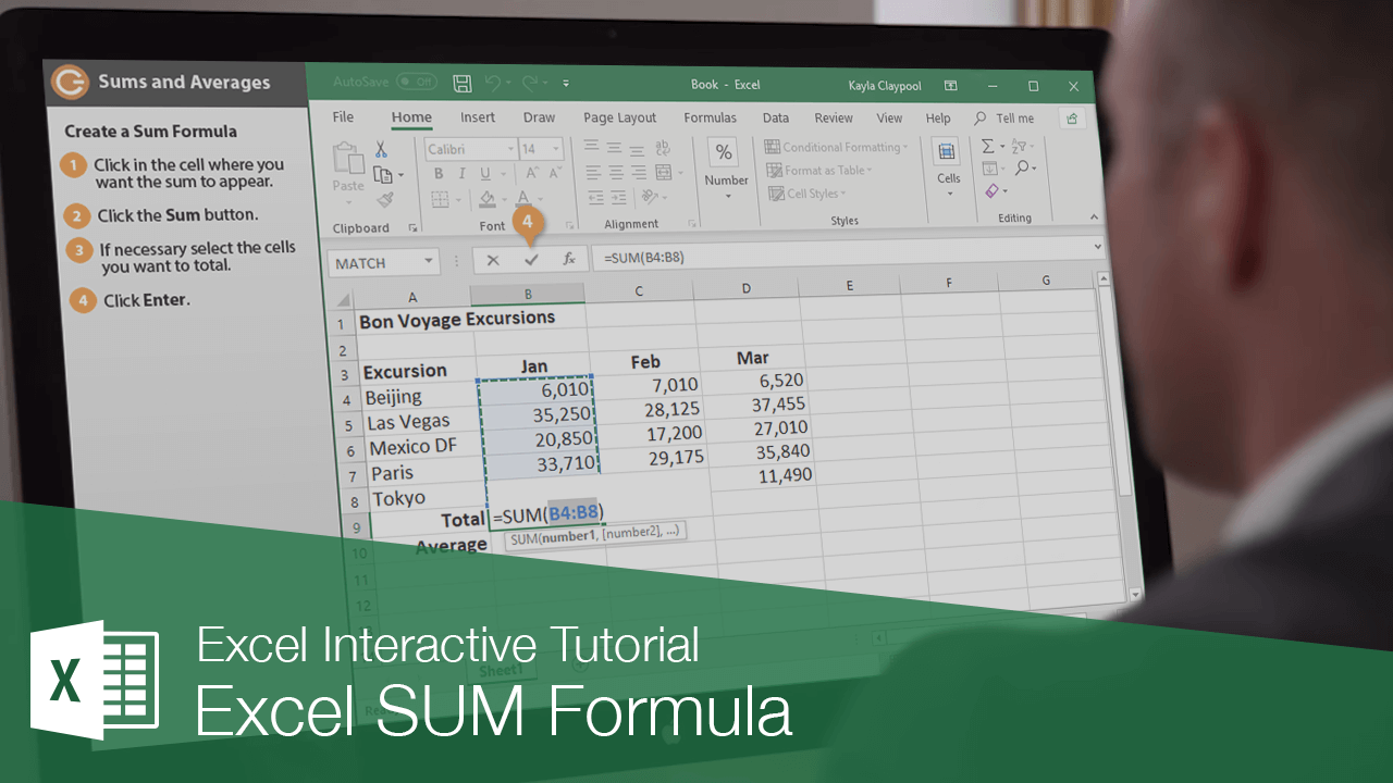
5 Simple Ways to Sum Totals in Excel Quickly

Summing up numbers in Excel is a fundamental skill, often used for everything from monthly budget calculations to complex financial analyses. While there are numerous methods to sum totals, knowing the quickest and most efficient ways can save you a significant amount of time, especially when dealing with large datasets. This post will explore five simple ways to sum totals in Excel quickly, ensuring you can breeze through your data work.
1. Using the AutoSum Feature

Excel’s AutoSum tool is a quick way to sum numbers without typing a formula.
- Select the cell below the column of numbers or to the right of the row where you want the sum.
- Go to the Home tab, click on ‘AutoSum’ in the ‘Editing’ group, or press Alt + = (Mac: Ctrl + =).
- Excel will automatically insert the SUM formula and highlight the range of cells to be summed.
- If Excel doesn’t select the right range, adjust it manually by dragging over the correct cells.
💡 Note: AutoSum also works for other functions like AVERAGE, COUNT, and MAX by selecting from its dropdown menu.
2. SUM Function

For more control over what you’re summing, you might prefer using the SUM function directly.
- In the cell where you want the total, type =SUM( or select it from the formula dropdown list.
- Select the range of cells you want to sum, or type them manually (e.g., =SUM(A1:A10)).
- Press Enter to complete the formula.
3. Quick Selection for Adjacent Cells

Sometimes, you just need to sum up nearby numbers quickly.
- Click the cell where you want the sum to appear.
- Hold down the Shift key, then click and drag over the cells you want to sum.
- Release the mouse button, then let go of the Shift key. Excel will display the sum in the status bar.
- If you want to enter this sum into a cell, go back to that cell, press ‘=’ and then Ctrl + Alt + V (Paste Special), choose ‘Values’ and hit Enter.
4. SUBTOTAL Function for Filtering Data

When working with filtered lists or tables, the SUBTOTAL function ensures you sum only visible cells:
- Type =SUBTOTAL(9, A1:A100), where 9 is the function number for SUM, and A1:A100 is the range.
- Unlike SUM, SUBTOTAL ignores hidden or filtered-out rows.
- It’s extremely useful in scenarios where you frequently filter data and want dynamic sums.
5. Table Summaries

Excel tables automatically calculate totals at the bottom, making it a straightforward process:
- Convert your range of data into a table by selecting it and pressing Ctrl + T.
- A row for totals will appear at the bottom. Click in the cell under the column where you want the sum.
- From the dropdown, choose ‘Sum’ from the list of functions provided.
- Excel will automatically update this sum as you add or modify data within the table.
💡 Note: Tables also provide features like automatic formatting, column headers that sort and filter, and easy data expansion.
In conclusion, knowing how to sum totals efficiently in Excel can greatly enhance your productivity. Whether you prefer the simplicity of AutoSum, the flexibility of direct functions like SUM and SUBTOTAL, or the dynamic nature of tables, Excel offers tools for every scenario. By mastering these quick methods, you'll not only save time but also make your data analysis tasks less tedious and more accurate.
Why isn’t AutoSum working for me?

+
AutoSum might not work if there are gaps in your data or if you’re trying to sum non-numeric values. Ensure your data is contiguous and the cells you’re summing contain numbers.
Can I use SUM on non-contiguous cells?

+
Yes, you can sum non-contiguous cells by holding down Ctrl and selecting each range or cell you want to include in the SUM formula.
How do I handle summing hidden or filtered cells?

+
Use the SUBTOTAL function which has the flexibility to include or exclude hidden or filtered cells based on the function number used.


