Excel Tips: Easily Retrieve Data from Another Sheet

In this comprehensive guide, we'll walk through the methods for efficiently retrieving data from one Excel sheet to another. Excel, a cornerstone of data management in many organizations, allows for complex data manipulation, which includes transferring data across different sheets within the same workbook. This post will explore various techniques that enhance productivity and accuracy in your data operations.
Why You Might Need to Pull Data from Another Sheet

Before we delve into the methods, understanding the reasons for needing to retrieve data from another sheet can provide context:
- Data Consolidation: Combining information from multiple sources into one coherent dataset.
- Report Creation: Pulling key figures from different sheets to compile a comprehensive report.
- Referencing: Referencing data without physically copying it, ensuring data integrity and maintaining a dynamic link.
Using Cell References

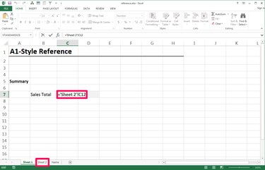
The simplest and most direct way to pull data from another sheet is by using cell references. Here’s how:
- Select the cell where you want the data to appear.
- Enter an equals sign (=) followed by the sheet name (preceded by an exclamation mark) and then the cell reference.

🔗 Note: Ensure the sheet name is correctly spelled, and if it contains spaces, use single quotes around the name.
The VLOOKUP Function

VLOOKUP is powerful for searching vertically through a column in a different sheet to retrieve data based on a key. Here’s the structure:
- VLOOKUP(lookup_value, table_array, col_index_num, [range_lookup])

Here’s an example:
| Step | Description |
|---|---|
| 1 | Select the cell where you want the result. |
| 2 | Start with =VLOOKUP( |
| 3 | Enter the value you’re looking for. |
| 4 | Select the range of cells to search (from the other sheet). |
| 5 | Specify the column number containing the data you need. |
| 6 | Choose whether you want an exact match (FALSE) or approximate match (TRUE). |
| 7 | Close the parenthesis and press Enter. |

The HLOOKUP Function

HLOOKUP works similarly to VLOOKUP but searches horizontally:
- HLOOKUP(lookup_value, table_array, row_index_num, [range_lookup])

INDEX and MATCH

The combination of INDEX and MATCH functions allows for a flexible way to look up and retrieve data without the limitations of VLOOKUP or HLOOKUP:
- INDEX(array, MATCH(lookup_value, lookup_array, [match_type]))
📌 Note: MATCH is used to locate the position of the lookup value, then INDEX uses that position to return the value from the specified array.
Indirect Function for Dynamic References

The INDIRECT function allows for dynamic references which can be useful when sheet names or cell references change:
- INDIRECT(“SheetName!” & “CellReference”)
This function is particularly handy when you need to reference cells based on values or other functions’ results.
Using Excel’s Advanced Query Tools

For complex data retrieval, especially in large datasets:
- Power Query: Import and transform data from various sources, including other sheets in your workbook.
- Get & Transform: Use this feature to automatically update data from different sources.
Summary of Data Retrieval Techniques

Having explored various techniques for retrieving data from one sheet to another in Excel, we can summarize:
- Cell References are straightforward but best for simple tasks.
- VLOOKUP/HLOOKUP are versatile for searching through columns or rows but have limitations regarding the search direction.
- INDEX and MATCH provide flexibility, particularly useful for 2-dimensional lookups.
- The INDIRECT function offers dynamic data referencing, useful for adapting to changes in sheet or cell names.
- Advanced Query tools like Power Query and Get & Transform are ideal for large, complex data manipulations.
Understanding these methods allows you to choose the most suitable approach based on your specific needs, enhancing data management efficiency, accuracy, and integration across different sheets within your Excel workbook.
Can I pull data from a different workbook using these methods?

+
Yes, you can. Use the same methods but include the full file path in your formula to reference cells in different workbooks. For example, =VLOOKUP(A1, ‘[AnotherWorkbook.xlsx]Sheet1’!A1:B100, 2, FALSE)
How do I ensure that my references update if I add or delete rows/columns in the source sheet?

+
Use absolute references (using signs) for your formulas, like =Sheet1!A1 to keep the reference fixed, or use Table functionality which updates automatically with data changes.
What happens if I rename the source sheet?

+
If you rename the source sheet after setting up your formulas, Excel will not automatically update those references. You’ll need to manually update your formulas to reflect the new sheet name, or use INDIRECT to dynamically reference sheet names.


