How to Freeze Excel Sheet Columns and Rows Easily

When working with large datasets in Microsoft Excel, keeping critical information visible while scrolling through extensive lists is vital for accuracy and efficiency. Freezing rows and columns is a feature that can significantly enhance your productivity by allowing you to anchor certain areas of your spreadsheet. In this comprehensive guide, we'll walk through the steps to freeze columns and rows in Excel, ensuring you can work smarter, not harder.
What is Freezing in Excel?

Freezing in Excel means locking rows and columns in place so they remain visible when you scroll through the worksheet. Here are the benefits:
- Enhanced readability: Keep headers or key rows/columns always in view.
- Efficiency: Reduces errors by having reference data on screen.
- Clarity: Easier to follow data relationships and patterns when referencing headers.
How to Freeze Columns

To freeze columns in Excel, follow these steps:
- Open your Excel workbook and select the worksheet you want to modify.
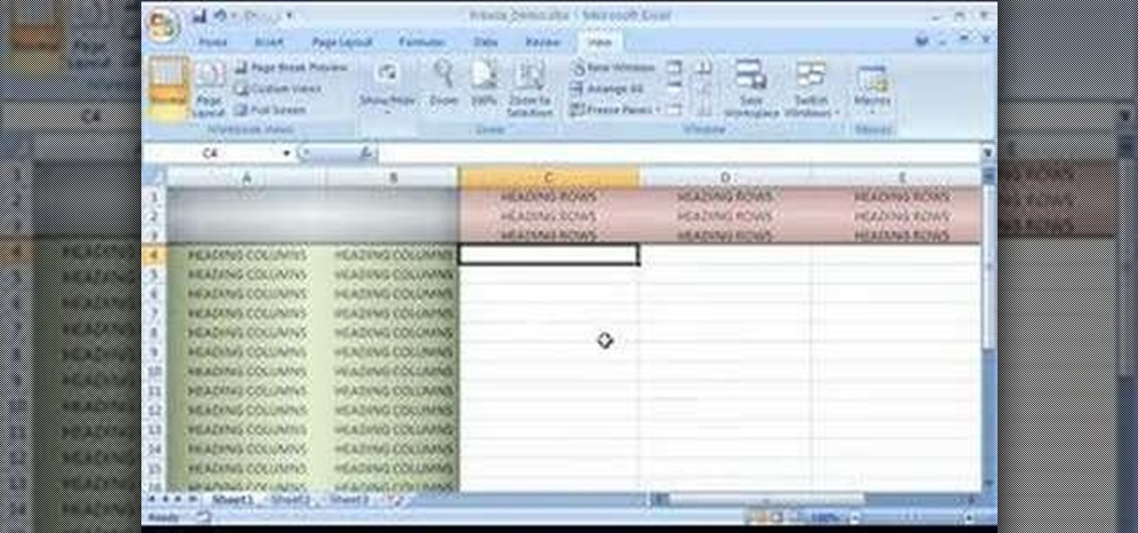
- Select the column immediately to the right of the column you wish to freeze.
📝 Note: Excel freezes columns to the left of the selected column.
- Go to the 'View' tab in the Ribbon.
- Click on 'Freeze Panes' in the 'Window' group.
- From the dropdown, choose 'Freeze Panes' to freeze the columns to the left of your current selection.
How to Freeze Rows

Similarly, to freeze rows:
- Select the row below the one you want to freeze.
- Go to the 'View' tab.
- In the 'Window' group, click 'Freeze Panes'.
- Choose 'Freeze Panes' from the dropdown to lock rows above the selected row.
Freezing Both Columns and Rows

If you want to freeze both columns and rows:
- Click the cell that is directly below the rows and to the right of the columns you want to freeze.
- Go to the 'View' tab and click 'Freeze Panes'.
- Select 'Freeze Panes' from the options to lock both columns to the left and rows above the cell.
Advanced Freezing Techniques

Excel offers some advanced options for freezing:
- Freeze First Column: Use 'Freeze First Column' to always keep the first column visible.
- Freeze Top Row: 'Freeze Top Row' keeps the first row fixed as you scroll.
Unfreezing Panes

To unfreeze panes:
- Navigate to the 'View' tab.
- In the 'Window' group, click on 'Freeze Panes'.
- Select 'Unfreeze Panes' to release all frozen panes.
Keyboard Shortcuts for Freezing

For power users, these shortcuts can streamline your workflow:
| Action | Windows | Mac |
|---|---|---|
| Freeze Panes | Alt + W, F, F | Option + View, then F, F |
| Unfreeze Panes | Alt + W, F, R | Option + View, then F, U |

Final Thoughts on Freezing Excel Panes

Mastering the ability to freeze columns and rows in Excel can save you time and reduce errors. By keeping key headers and reference points in view, you'll be able to navigate large datasets with ease, ensuring your work is both accurate and efficient. Remember to use these techniques when working with extensive data, for data analysis, or when presenting data in meetings where scrolling through information is frequent.
💡 Note: While freezing panes is a useful feature, overusing it can clutter your screen. Freeze only what's necessary to maintain clarity and simplicity.
What happens if I scroll after freezing panes?

+
Scrolling will move the active cell, but the frozen panes will remain fixed, allowing you to see headers or reference columns/rows regardless of your position on the sheet.
Can I freeze panes in the middle of the sheet?

+
Yes, by selecting a cell or column/row in the middle of your worksheet, you can freeze sections of the sheet. Excel will freeze the parts to the left and above the selection.
Are frozen panes visible when I print my sheet?

+
Frozen panes do not affect printing. They are solely for on-screen navigation. For print, consider repeating rows or columns.
How do I know if panes are frozen in a workbook?

+
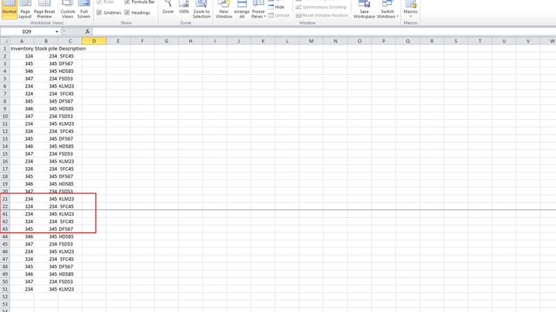
Look for the frozen lines on the screen, which will appear as thick lines separating the fixed areas from the scrollable sections.


