Find Duplicate Names in Excel Fast and Easy

When dealing with large datasets in Excel, one common task is identifying duplicate entries. Whether you're managing customer databases, inventory lists, or any other records, finding duplicate names can be essential to maintain data integrity and improve efficiency. In this guide, we'll explore easy and fast methods to find duplicate names in Excel, ensuring you can clean your spreadsheets with minimal hassle.
Why You Need to Find Duplicates in Excel

Before we dive into the methods, let’s briefly cover why detecting duplicates in Excel is important:
- Data Cleansing: Duplicates can distort data analysis by inflating counts and affecting calculations.
- Accuracy: Removing duplicates ensures that your data represents the real-world scenario accurately.
- Efficiency: Identifying and removing duplicates can save storage space and make spreadsheets easier to work with.
Using Conditional Formatting to Highlight Duplicates

Excel’s Conditional Formatting feature is a powerful tool that can instantly highlight duplicate names:
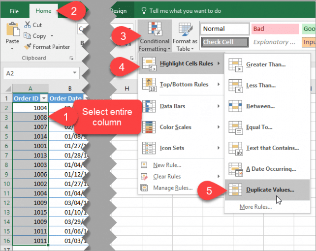
- Select the range of cells where you want to check for duplicates.
- Go to the Home tab, then click on Conditional Formatting > Highlight Cells Rules > Duplicate Values.
- Choose the format in which you want to highlight the duplicates (e.g., light red fill with dark red text).
💡 Note: This method is visual and won’t remove or sort the duplicates, but it provides a clear indication of where duplicates are located in your dataset.
Using Formulas to Identify Duplicate Names

If you need a more technical approach, you can use Excel formulas:
COUNTIF Formula

To count the number of times a name appears:
=COUNTIF(range, criteria)
- Replace range with the column where you’re checking for duplicates.
- Replace criteria with the cell containing the name you’re checking.
Use this formula in a new column, and any value greater than 1 will indicate a duplicate entry.
IF and EXACT Formulas

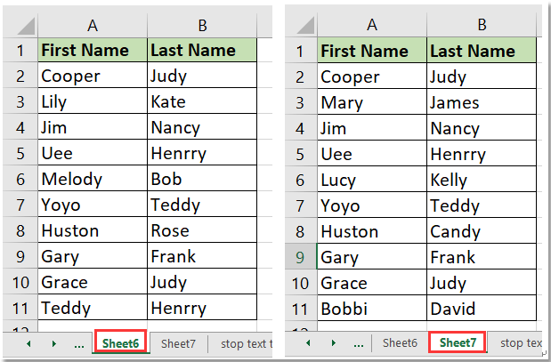
To list duplicate names side by side:
=IF(EXACT(A2,A3),A2,“”)
Here:
- A2 and A3 are adjacent cells. Adjust according to your data layout.
- If the names match exactly, the formula will display the duplicate name; otherwise, it returns an empty string.
Advanced Technique: Using Excel Power Query

For those dealing with large datasets, Power Query offers a more dynamic way to handle duplicates:
- Select your data range or table.
- Go to the Data tab > Get & Transform Data > From Table/Range.
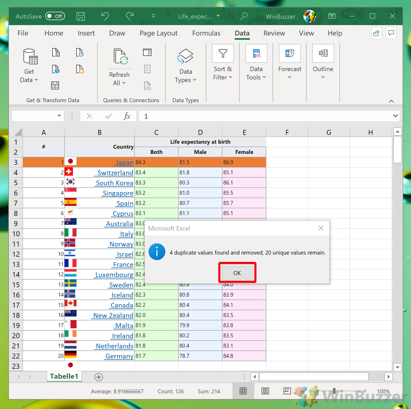
- In the Power Query Editor, click on Home > Remove Rows > Remove Duplicates.
- Close and load the data back into Excel.
💡 Note: Power Query transforms data before loading it back into Excel, which means your original data remains unchanged until you apply the changes. This is useful for exploring different scenarios or when you need to revert changes.
| Method | Advantage | Disadvantage |
|---|---|---|
| Conditional Formatting | Easy to use, visually highlights duplicates | Doesn't sort or remove duplicates |
| Formulas | Flexible, can be automated in macros | Can be complex for large datasets, time-consuming to set up |
| Power Query | Handles large datasets efficiently, allows for data transformation | Requires some learning curve, changes are reversible but require re-application |

To summarize, we've covered three primary methods to detect duplicate names in Excel:
- Conditional Formatting: Quick visual identification.
- Formulas: For a more detailed analysis or automated approach.
- Power Query: Best for large datasets and when you need to transform your data before analysis.
Each method has its place in Excel data management, allowing you to choose based on your specific needs and dataset size.
Can I remove duplicates without altering my original data?

+
Yes, you can use Power Query to remove duplicates without altering your original dataset. After performing transformations in Power Query, you can preview the changes and then load the modified data into a new location, leaving your original data intact.
What if my data contains names formatted differently?

+
Excel’s text functions like TRIM(), UPPER(), LOWER(), or PROPER() can standardize name formats before checking for duplicates. Also, consider using case-insensitive comparisons in your formulas.
How can I highlight only the first occurrence of each duplicate?

+
To highlight only the first instance, you might need to combine conditional formatting with a formula. A formula like =COUNTIF(A$2:A2,A2)=1 would mark the first occurrence, while subsequent matches would not be highlighted.
Does Excel have a built-in function to check for duplicates in multiple columns?

+
Excel’s built-in “Remove Duplicates” feature allows for checking duplicates across multiple columns at once. However, for highlighting, you would need to combine or adjust formulas or use advanced filtering techniques.


