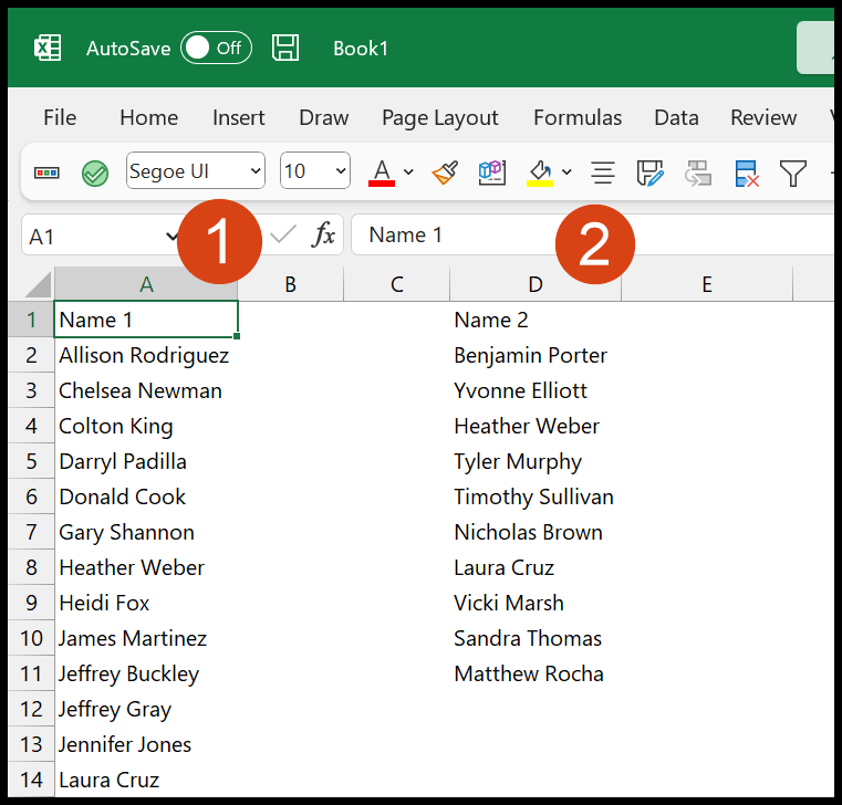
5 Simple Ways to Compare Excel Columns in Seconds

Comparing Excel columns efficiently can transform the way you analyze data, saving you time and enhancing accuracy. In this guide, we'll delve into five straightforward methods that can help you compare Excel columns in mere seconds, revolutionizing your workflow.
Understanding the Importance of Column Comparison

Before diving into the techniques, let’s briefly understand why comparing columns in Excel is crucial:
- Data Validation: Ensuring the data across columns is consistent.
- Identifying Duplicates: Spotting entries that appear more than once.
- Error Detection: Finding discrepancies or mistakes in data entry.
💡 Note: Regular column comparison can lead to a cleaner dataset, making data analysis more straightforward.
1. Using Conditional Formatting for Visual Comparison


Conditional Formatting is a powerful tool in Excel that visually differentiates data based on specific criteria. Here's how you can use it:
- Select the Columns: Highlight the columns you want to compare.
- Navigate to Conditional Formatting: From the 'Home' tab, select 'Conditional Formatting'.
- Choose a Rule: Go for 'Highlight Cells Rules' > 'Duplicate Values' or 'Unique Values'.
- Set the Format: Choose the colors or styles you want to apply to highlight the differences.
📚 Note: Conditional Formatting changes how data appears but does not alter the actual data in cells.
2. VLOOKUP Function for Detailed Comparison

VLOOKUP is invaluable when comparing columns, especially when you need to check if items from one column exist in another:
=VLOOKUP(A2, B:B, 1, FALSE)
- A2: The cell to look up from the first column.
- B:B: The entire column to search in.
- 1: Indicates the column in which to find the match.
- FALSE: For an exact match.
🧩 Note: VLOOKUP is best for one-to-one comparisons; for many-to-many comparisons, consider other functions.
3. Pivot Tables for Cross-Column Analysis

Pivot tables offer a dynamic way to compare data across multiple columns:
- Create a Pivot Table: Select your data range and insert a pivot table.
- Add Fields: Drag your columns into ‘Row Labels’, ‘Column Labels’, and ‘Values’ as needed.
- Filter and Sort: Use filters and sorting to highlight differences or commonalities.
📈 Note: Pivot tables can be complex but provide a rich toolset for data analysis.
4. Using COUNTIF for Simple Duplicates Detection

The COUNTIF function can quickly identify how many times a value appears:
=COUNTIF(B:B, A2)
- A2: The cell to count occurrences from.
- B:B: The range to check for duplicates.
🔍 Note: COUNTIF is excellent for quick checks but not for extensive data analysis.
5. Advanced Filtering for In-Depth Analysis

Advanced filtering allows for more refined searches across columns:
- Go to Data: Click ‘Data’ and then ‘Advanced’ from the ‘Sort & Filter’ group.
- Set Criteria: Define the criteria range in the ‘List range’ field.
- Apply Filter: Click ‘OK’ to filter the data according to your conditions.
🔎 Note: Advanced filtering is especially useful when dealing with large datasets where simple methods might fall short.
These techniques offer versatile methods to compare Excel columns. Whether you're looking to validate data, find duplicates, or perform in-depth analysis, there's an approach for every scenario. By implementing these strategies, you'll enhance your ability to manage and interpret data, ensuring your Excel work becomes more efficient and less error-prone.
What’s the fastest way to compare two columns for duplicates?

+
Use the =COUNTIF(range, criteria) formula to quickly find how many times a value appears across columns.
Can I use these methods on multiple columns simultaneously?

+
Yes, all methods can be adapted to compare several columns at once, although pivot tables are particularly effective for this.
What if I need to compare columns from different sheets?

+
You can use formulas like VLOOKUP or INDEX MATCH to compare columns from different sheets by referencing their specific cells or ranges.


