5 Simple Ways to Sum Numbers in Excel Quickly

Understanding the Basics of Excel’s SUM Function

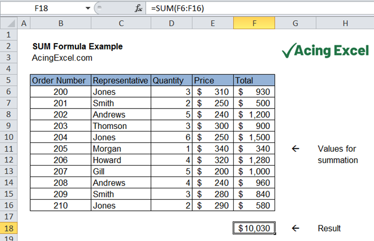
Excel’s SUM function is an indispensable tool for anyone dealing with numbers. It allows you to quickly sum up values in a range, column, or row. Here’s how you can start:
- Select the cell where you want the sum to appear.
- Type “=SUM(” followed by the range of cells you want to sum, for example, “=SUM(A1:A10)” and then close the parenthesis.
- Press Enter, and Excel will calculate the sum for you.

Using AutoSum for Quick Results

AutoSum is one of the most convenient features in Excel for summing numbers with minimal effort:
- Select the cell where you want the sum to appear, ideally adjacent to your data.
- Click on the AutoSum icon on the Home tab or press Alt + =.
- Excel will automatically detect the range to sum and suggest a formula. If the suggestion is incorrect, you can adjust the range by clicking and dragging the dotted line around the suggested cells.

Summing Across Sheets with 3D References

Summing across multiple sheets or tabs in an Excel workbook can be a bit tricky, but here’s how you do it:
- Go to the cell where you want the sum to appear.
- Start typing the SUM function: “=SUM(”.
- Type the first cell reference followed by a colon (e.g., “=SUM(Sheet1!A1:).
- Holding the Shift key, click on the last sheet you want to include in the sum.
- Excel will fill in the 3D reference for you, e.g., “=SUM(Sheet1:Sheet3!A1)”.
💡 Note: The sheets must be named consistently for the 3D reference to work correctly. If they are not, you may need to adjust them manually or rename them.
Conditional Summation with SUMIF/SUMIFS

When you need to sum numbers based on certain criteria, SUMIF or SUMIFS come in handy:
- SUMIF: Use when you need to sum cells that meet a single criterion.
- SUMIFS: Use when you need to sum cells that meet multiple criteria.
Using SUMIF

Here’s how you can use SUMIF to sum cells that meet one criterion:
- Type “=SUMIF(” and provide three arguments: the range to apply the criteria, the criteria itself, and the range of cells to sum.
- For example, “=SUMIF(A1:A10, “>50”, B1:B10)” sums all values in column B where column A has numbers greater than 50.
Using SUMIFS

With SUMIFS, you can sum values based on multiple criteria:
- Type “=SUMIFS(” and provide at least three arguments: the range to sum, the first criteria range, the first criteria, and so on for additional criteria.
- Example: “=SUMIFS(A1:A10, B1:B10, “>50”, C1:C10, “Product A”) sums values in column A where column B has values greater than 50 and column C is “Product A”.
Using Tables for Dynamic Summation

Excel tables offer dynamic functionality for summation, allowing data to expand without having to adjust your sum formula:
- Convert your range of data into a table by selecting any cell within it and pressing Ctrl + T.
- Use the total row to automatically sum up columns. You can choose what function to apply to each column.
- Formulas will automatically adjust when you add new data to the table, making your workbook more adaptable.
💡 Note: Using tables not only makes summing dynamic but also improves the readability and organization of your data.
In this post, we've covered several efficient methods for summing numbers in Excel. Each method serves different needs, from basic summation to more complex conditional summing. Understanding these techniques will not only save you time but also make your data analysis more accurate and powerful.
Can I sum cells that contain text and numbers?

+
Yes, but only the numeric values will be summed. Text in cells is ignored by Excel’s SUM function.
What if I want to sum only visible cells after filtering?

+
Use the SUBTOTAL function with function_num argument 9 or 109 to sum only the visible cells after filtering.
Can SUMIF handle dates as criteria?

+
Yes, SUMIF can use dates as criteria, but you must ensure they are formatted correctly as dates in Excel.
How do I sum numbers across different workbooks?

+
You can reference cells from other workbooks using external references, like ‘=[WorkbookName]SheetName!A1:A10’ within your SUM function.


