5 Ways to Use Formulas in Excel Quickly

Excel is an incredibly versatile tool that's used by millions for data analysis, reporting, and much more. While many people know the basic functionality, diving deeper into Excel's capabilities can dramatically enhance productivity. This guide will take you through five innovative ways to use formulas in Excel to speed up your work, making you more efficient and effective in handling data.
1. Flash Fill: The Smart Formula Helper

Flash Fill is not a formula, but it’s an Excel feature that can act like one by automatically filling in data based on patterns it recognizes. This tool can save hours when dealing with repetitive data entry.
- To Use: Start typing the pattern you want Excel to recognize in a column next to your data, hit Enter, then click on the Flash Fill button in the Data Tools group on the Data tab.
- Example: If you have a column with names in the format "LastName, FirstName" and you want to separate them into two columns, simply type "FirstName" in one cell and "LastName" in another, then use Flash Fill to complete the task.
💡 Note: Flash Fill might not always recognize your desired pattern, so checking its results is recommended.
2. Array Formulas: Batch Processing at Its Best

Array formulas allow you to perform multiple calculations on one or more items in an array. They’re especially powerful for complex calculations that can’t be done with single-cell formulas.
- To Use: Enter the formula and press Ctrl+Shift+Enter instead of just Enter. Excel will enclose the formula in curly braces {} to signify it's an array formula.
- Example: Suppose you want to sum the product of two arrays (A2:A10 * B2:B10). You'd write the formula as =SUM(A2:A10*B2:B10) and press Ctrl+Shift+Enter.
| Function | Use Case |
|---|---|
| SUMPRODUCT | Multiplying two sets of data and summing the result |
| TRANSPOSE | Flipping data from rows to columns or vice versa |
| LARGE | Returning the nth largest value in a range |

3. Dynamic Named Ranges: Adaptable Formulas

Dynamic named ranges automatically adjust when data is added or removed, making your formulas always work with the latest data set.
- To Use: Use the OFFSET and COUNTA functions to create a dynamic range. Name this range through the Name Manager or by using Define Name.
- Example: Let’s say you have sales data in A2:A30, but you add more data every month. You could name this range "Sales" by defining it as =OFFSET($A$2,0,0,COUNTA($A:$A)-1,1). Now your SUMIF formula using this range will automatically include all data.
4. Conditional Formatting Formulas: Visual Data Analysis

While conditional formatting isn’t a formula per se, using formulas within it can significantly enhance data visualization and analysis.
- To Use: Click on Conditional Formatting in the Home tab, choose "New Rule," then select "Use a formula to determine which cells to format."
- Example: To highlight cells where the value is greater than the average, you would use a formula like: =A2>AVERAGE($A$2:$A$1000).
⚠️ Note: Conditional formatting rules can impact the performance of large spreadsheets, use them judiciously.
5. IF, AND, OR: Advanced Logical Functions

These logical functions allow for complex decision-making within your spreadsheets, enabling you to construct powerful conditional statements.
- To Use: Combine these functions to create intricate conditions. Use IF for single conditions, AND to check if all conditions are met, and OR for when at least one condition is true.
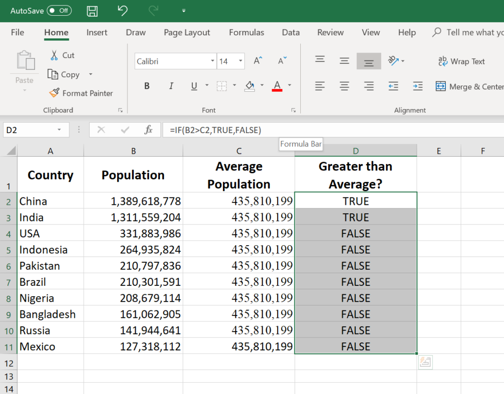
- Example: To calculate a bonus based on performance and attendance, you might use: =IF(AND(A2>500,B2>=10),100,IF(OR(A2>400,B2>=8),50,0))
In summary, by mastering these five techniques, you can leverage Excel's formula capabilities to streamline your work, make complex calculations simpler, and visually analyze data effectively. From Flash Fill's smart pattern recognition to the power of array formulas and dynamic named ranges, Excel offers numerous ways to boost productivity. Logical functions like IF, AND, OR provide the basis for sophisticated decision-making within your data, enhancing both the accuracy and efficiency of your work.
What’s the difference between a regular formula and an array formula?

+
A regular formula performs calculations on individual cells, whereas an array formula can handle multiple cells or ranges simultaneously, performing calculations on entire sets of data.
Can I revert a dynamic range if data is removed?

+
No, dynamic ranges adjust automatically to include or exclude data based on conditions set by formulas like OFFSET. If data is removed, the range will update to reflect that. However, if you need to revert this change, you would need to manually adjust the named range or reset it in the Name Manager.
Why isn’t Flash Fill working as expected?

+
Flash Fill might not work if the pattern you’re trying to create is too complex or if there are inconsistencies in your data. Ensure the pattern is clear, consistent, and immediately adjacent to the column containing the data you’re formatting.