5 Simple Steps to Master VLOOKUP in Excel

Mastering VLOOKUP in Microsoft Excel can significantly enhance your data analysis capabilities. Whether you're dealing with large datasets or simple lists, VLOOKUP allows you to search for specific information with ease. This guide will take you through the steps needed to understand and use VLOOKUP effectively.
Understanding VLOOKUP

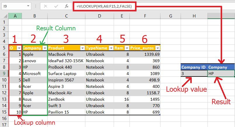
VLOOKUP, short for Vertical Lookup, is a function in Excel that searches for a value in the leftmost column of a table and returns a corresponding value from another column within the same row. Here are the basic components you need to know:
- Lookup_value - The value to search for in the first column of your table.
- Table_array - The range of cells that contain the data.
- Col_index_num - The column number in the table from which to retrieve the value.
- Range_lookup - A logical value (TRUE for approximate match or FALSE for exact match).
Step-by-Step Guide to Using VLOOKUP

1. Prepare Your Data

First, ensure your data is organized in a tabular format with the lookup column on the left side. Here’s what your data should look like:
| Employee ID | Employee Name | Department | Salary |
|---|---|---|---|
| 101 | Jane Doe | Marketing | 45000 |

This table structure is essential for VLOOKUP to work properly.
2. Enter the VLOOKUP Formula

To use VLOOKUP, click on the cell where you want the result to appear and type:
=VLOOKUP(lookup_value, table_array, col_index_num, [range_lookup])
Replace the placeholders with actual values from your data:
- Lookup_value: The ID you want to look up, for example, A1 if your lookup column contains IDs.
- Table_array: The range of cells containing your table, like B2:E100.
- Col_index_num: The column number from where you want to pull the data (2, 3, or 4 in the example).
- Range_lookup: TRUE for an approximate match or FALSE for an exact match.
📝 Note: When using a dynamic or named range for your table array, remember to adjust the formula accordingly.
3. Error Checking and Troubleshooting

Sometimes VLOOKUP might not work as expected. Here are some common issues:
- #N/A Error: The lookup value is not in the first column of the table array or there is no match.
- #REF! Error: The column index number is greater than the number of columns in the table array.
- Wrong or Unexpected Results: Check if the lookup column is sorted in ascending order for approximate matches.
4. Advanced Tips for VLOOKUP Mastery

- Use Named Ranges for better readability and easier management of your Excel workbook.
- Combine VLOOKUP with Other Functions like IFERROR to handle errors gracefully:
=IFERROR(VLOOKUP(A1,B2:E100,2,FALSE),“Not Found”)
5. Practice and Experiment

The best way to master VLOOKUP is through consistent practice. Here are some exercises to help you:
- Create a dummy dataset and try to look up various values.
- Practice error handling and troubleshooting.
- Experiment with different range_lookup values to see how they affect your results.
As you apply these steps, you'll gain a deeper understanding of how VLOOKUP can be used to streamline your work in Excel. Remember, mastering any tool takes time and practice, so keep refining your skills by experimenting with real-world scenarios or sample data sets.
What does #N/A error mean in VLOOKUP?

+
The #N/A error in VLOOKUP typically means that the lookup value does not exist in the first column of the table array.
Can VLOOKUP search for data in different sheets?

+
Yes, VLOOKUP can reference data across different sheets. You would specify the sheet name in your table array reference, like Sheet2!A1:D100.
How do I perform a case-sensitive VLOOKUP?

+
VLOOKUP is not inherently case-sensitive. For case-sensitive lookups, you might need to combine VLOOKUP with other functions or use an array formula.


