5 Simple Ways to Add If Conditions in Excel

In Excel, conditional formatting and formulas are powerful tools to streamline your data processing. Adding if conditions can help you analyze, organize, and manipulate data based on specific criteria, making your spreadsheets more dynamic and useful. This post will explore five simple methods to integrate if conditions into your Excel spreadsheets, from basic to advanced techniques.
1. Using IF Function

The most straightforward method to add conditional logic in Excel is by using the IF function. This function allows you to test a condition and return one value if the condition is true and another if it is false.
IF(logical_test, value_if_true, value_if_false)
- logical_test: The condition you want to check.
- value_if_true: The result if the condition is true.
- value_if_false: The result if the condition is false.
Example:
=IF(A2>100, “Above Target”, “Below Target”)
If the value in cell A2 is greater than 100, it will display “Above Target”; otherwise, it will show “Below Target”.
2. Combining Multiple IF Conditions with AND/OR

Excel allows you to combine multiple conditions within a single IF statement using logical operators like AND or OR.
- AND: All conditions must be true for the overall condition to be true.
- OR: At least one condition must be true for the overall condition to be true.
Example:
=IF(AND(A2>100, B2=“Yes”), “Meets Both”, IF(OR(A2>100, B2=“Yes”), “Meets Either”, “No Match”))
3. Nested IF Functions

Sometimes, a simple IF function isn’t enough. You can use nested IF functions for more complex conditions, where one IF statement sits inside another.
=IF(A2>100, “Above Target”, IF(A2>50, “Near Target”, “Below Target”))
Here, Excel first checks if A2 is greater than 100, then 50, and gives different outputs based on the nested conditions.
4. Using IF with Other Functions

The IF function can be paired with other Excel functions to create more sophisticated formulas. For instance, combining IF with VLOOKUP, SUMIF, or AVERAGEIF can yield powerful results.
Example with VLOOKUP:
=IF(VLOOKUP(A2,lookup_table,2,FALSE) = “Approved”, “Yes”, “No”)
This formula checks if the result of a VLOOKUP equals “Approved” and returns “Yes” or “No” accordingly.
5. Conditional Formatting Based on IF Logic

Although not a formula, conditional formatting can visually highlight cells based on conditional logic:
- Select the range of cells.
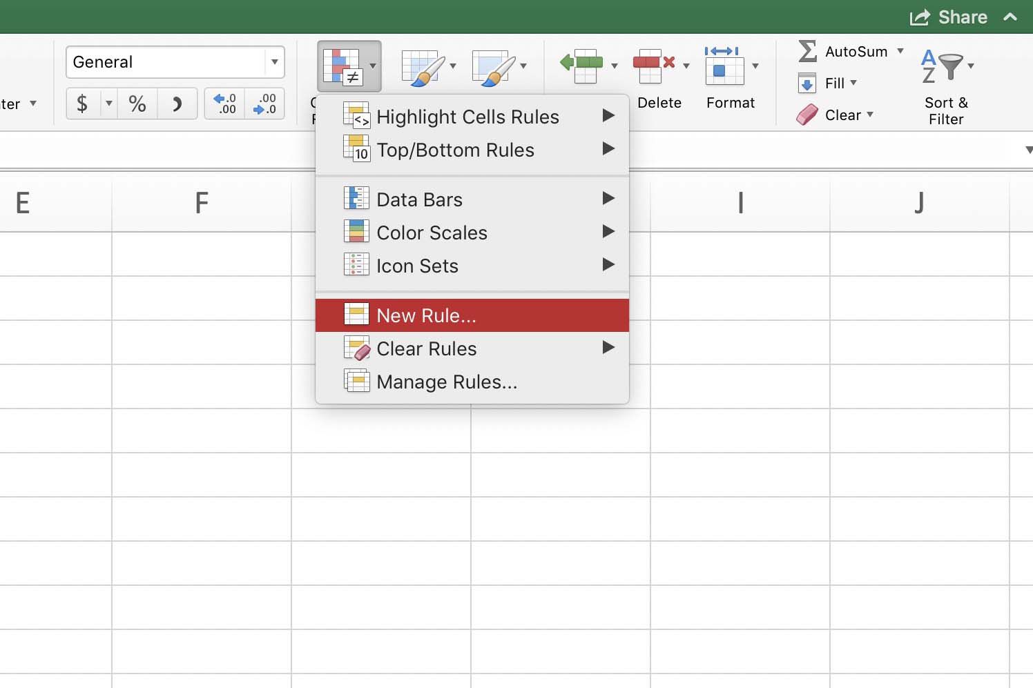
- Go to Home > Conditional Formatting > New Rule > Use a formula to determine which cells to format.
- Enter a formula similar to
=$A2>100. - Set the formatting options and click OK.
This will highlight cells in the selected range where the condition is met, such as cells containing values above 100.
To sum up, these five techniques for incorporating if conditions in Excel can significantly enhance your data analysis capabilities. From simple IF statements to complex nested formulas and conditional formatting, understanding these methods allows for more effective data manipulation and visual representation. With these skills, you can make Excel work smarter for you, tailoring your spreadsheets to meet specific conditions and highlighting critical data points instantly.
What is the difference between AND and OR in Excel?

+
AND requires all conditions to be true for the overall condition to be true, while OR requires at least one condition to be true.
Can you use more than two conditions with the IF function?

+
Yes, by nesting IF functions or combining them with AND or OR functions.
How can conditional formatting be used with IF logic?

+
By using the ‘Use a formula to determine which cells to format’ option in Excel’s conditional formatting rules, you can apply formatting based on any IF condition.
Is there a limit to how many IF functions can be nested?

+
Excel 2016 and later versions allow up to 64 nested IF functions, but it’s often better to use CHOOSE or LOOKUP functions for readability and performance.


