5 Easy Ways to Add Color in Excel Sheets

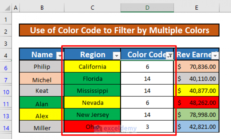
Adding color to your Excel sheets can dramatically enhance their readability, visual appeal, and overall impact. Whether you're managing a large dataset, creating an informative report, or simply organizing your work, the strategic use of color can help in highlighting key information, distinguishing between different types of data, and making navigation through spreadsheets more intuitive. Here, we'll explore five easy ways to add color to Excel, ensuring that your spreadsheets are not only functional but also visually engaging.
1. Using Fill Color

The most straightforward method to add color to your Excel sheet is by using the Fill Color option:
- Select the cell, row, or column you want to color.
- Go to the Home tab.
- Click on the Fill Color icon, which appears as a paint bucket.
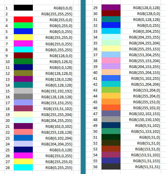
- Choose your color from the palette or customize it using the More Colors option.

💡 Note: Remember to use fill colors sparingly. Overuse can make your spreadsheet hard to read.
2. Conditional Formatting for Automatic Color Application

Conditional Formatting is a dynamic tool for coloring cells based on their content:
- Select the cells or range where you want to apply conditional formatting.
- Navigate to Home > Conditional Formatting.
- Choose a rule from options like Highlight Cells Rules, Top/Bottom Rules, or Color Scales.
- Set the conditions for when the color should be applied. For example, highlight cells greater than a certain number in red.

💡 Note: Conditional formatting is perfect for instantly identifying outliers or trends in your data.
3. Using Themes for a Coordinated Color Scheme

Excel provides various themes that can give your spreadsheet a consistent and professional look:
- Go to Page Layout > Themes.
- Select from a variety of pre-set themes that will apply coordinated color schemes, fonts, and effects throughout your document.
By using themes, you ensure that your colors complement each other, making your Excel sheet visually cohesive.

4. Manual Cell Formatting with Font and Border Color

In addition to fill color, you can manually adjust the font and border colors to highlight specific data points or add structure:
- For font color: Select the text, go to Home > Font Color, and pick a color.
- For borders: With cells selected, click on Home > Borders > Line Color to choose your color, then click Borders again to select the border style.
5. Creating a Data Bar or Icon Sets

Data Bars and Icon Sets provide a graphical representation of your data’s value or status:
- Select the range for which you want to add Data Bars or Icons.
- Under Home > Conditional Formatting > Data Bars or Icon Sets, choose the type you want.
This method visually represents data values directly within cells, making it easier to understand at a glance.

In summary, color in Excel sheets can transform your data from mundane to mesmerizing. From simple fill colors to complex conditional formatting, each method offers unique advantages for data presentation. Choose the approach that best suits your data visualization needs, keeping in mind that clarity and purpose should guide your color choices. With these techniques, your spreadsheets will not only serve as data storage but will also communicate information more effectively, making your work stand out.
Can I use more than one color in a single cell?

+
Yes, through conditional formatting, you can apply multiple color rules to a cell. However, only one condition can be true at a time, displaying that specific color.
How do I remove color from a cell?

+
To remove color, select the cell or range, go to the Home tab, click on Fill Color or Font Color, and choose “No Fill” or “Automatic” respectively.
Will adding color to my Excel sheet affect its performance?

+
While adding color won’t significantly slow down modern versions of Excel, an overuse of conditional formatting or intricate styles might impact performance in very large spreadsheets.


