5 Easy Ways to Highlight Duplicates in Excel Sheets

In the bustling world of data analysis, the task of spotting and dealing with duplicates in an Excel spreadsheet can often become a tedious chore. However, Excel provides us with several tools that can make this process much smoother and more efficient. Here, we will explore 5 easy ways to highlight duplicates in Excel that not only save time but also help in maintaining data integrity.

Understanding Duplicates

Before diving into the methods, it’s vital to understand what constitutes a duplicate in Excel. Typically, duplicates refer to cells or sets of cells within your dataset that contain identical data. This could range from simple text, numbers, or entire rows. Recognizing duplicates is essential for:

• Data Cleaning: To ensure your dataset is clean and error-free.
• Data Analysis: Preventing skewed results due to repeated entries.
• Reporting: Ensuring accuracy in reports where duplicate entries could mislead stakeholders.

Method 1: Conditional Formatting

Excel’s Conditional Formatting feature is your first line of defense against duplicates. Here’s how to use it:

1. Select the range of cells where you want to check for duplicates.
2. Go to the ‘Home’ tab, click on ‘Conditional Formatting’, and then ‘Highlight Cells Rules’.
3. Select ‘Duplicate Values’.
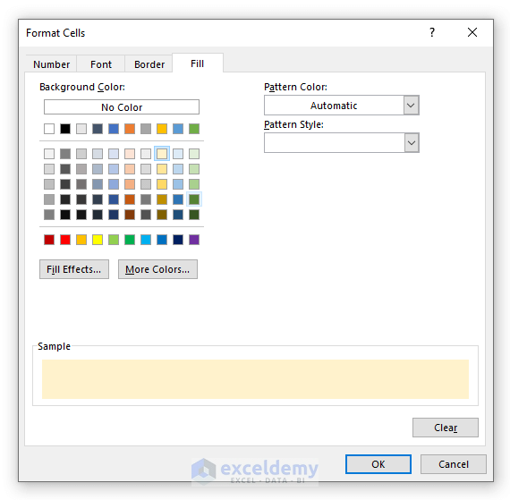
4. Choose the format with which you want to highlight duplicates (e.g., color).

💡 Note: Conditional Formatting can slow down large spreadsheets. Use it wisely, or consider clearing formatting after your work is done.

Method 2: Using Formulas

For those who prefer a more technical approach, formulas can be your ally. Here’s how you can highlight duplicates using formulas:

Counting Duplicates with COUNTIF

Use the following formula to highlight duplicates based on cell values:

=COUNTIF(A:A,A1)>1

Highlighting Whole Rows with Multiple Criteria

To highlight duplicate rows, use this formula in conditional formatting:

=COUNTIFS(A:A,A2,B:B,B2,C:C,C2)>1

Replace column letters with those that correspond to your data. Format the result with conditional formatting to highlight the entire row.

Method 3: Excel’s Advanced Filter

Excel’s Advanced Filter option allows you to filter out duplicates:

1. Select your dataset, go to ‘Data’ > ‘Advanced’.
2. Choose ‘Copy to another location’, and under ‘Unique records only’, check the box.
3. Excel will filter and copy only unique records to the specified location, leaving you with the duplicates highlighted.

Method 4: Using Power Query

For users dealing with larger datasets, Power Query (part of Excel since 2013) provides robust duplicate handling:

1. Select your data range, go to the ‘Data’ tab, and click ‘From Table/Range’.
2. In the Power Query Editor, navigate to ‘Home’ > ‘Remove Rows’ > ‘Remove Duplicates’.
3. This will keep only the unique rows. You can then load this data back into Excel with duplicates removed or highlighted as needed.

Method 5: PivotTables

PivotTables aren’t just for summarizing data; they can be used to spot duplicates:

1. Create a PivotTable from your dataset.
2. Drag the column you want to check for duplicates to both the ‘Row’ and ‘Value’ areas.
3. In the value field settings, set it to ‘Count’. Now, you can see which entries are repeated.

Each of these methods has its advantages, making it suitable for different data sizes and user preferences. Whether you're a beginner or an advanced user, there's a way for you to manage duplicates efficiently in Excel.

Summarizing the journey through Excel's capabilities to highlight duplicates, we've seen various techniques from simple to sophisticated. Remember, the choice of method depends on your dataset's complexity, your familiarity with Excel, and your intended use of the data. Whether it's for cleaning data, preparing reports, or enhancing data analysis, these tools ensure that your work remains accurate and your datasets are well-managed.

What happens if I have multiple duplicate values in Excel?

+

Excel will highlight all instances of duplicate values within the selected range using conditional formatting. If you are using COUNTIF or similar formulas, they will show a count greater than one for each duplicate entry.

Can I remove duplicates in Excel instead of just highlighting them?

+

Yes, you can remove duplicates using the ‘Remove Duplicates’ tool under the ‘Data’ tab or by using Power Query to keep only unique records. These methods allow you to either remove duplicates entirely or to keep one instance of each unique entry.

How can I highlight duplicates across different sheets?

+

While Conditional Formatting and COUNTIF formulas work within a single sheet, to highlight duplicates across sheets, you’ll need to consolidate your data or use Power Query to join datasets from multiple sheets and then apply the same techniques to the consolidated data.

Is there a way to highlight exact matches in rows across multiple columns?

+

Yes, you can use formulas like COUNTIFS or create complex conditional formatting rules to check for duplicates across multiple columns in a row. However, for large datasets, Power Query might be more efficient.

What are the limitations of these methods for highlighting duplicates in Excel?

+

Conditional Formatting can slow down Excel with large datasets, COUNTIF formulas might be less efficient for extensive data, and Power Query, while powerful, requires a learning curve. Also, cross-sheet highlighting requires data consolidation first.